doi:10.4236/ajor.2011.13012 Published Online September 2011 (http://www.SciRP.org/journal/ajor)
Two-Stage Ordering Policy under Buyer’s
Minimum-Commitment Quantity Contract
Hsi-Mei Hsu, Zi-Yin Chen
Department of Industrial Engineering & Management, National Chaio Tung University, Hsinchu, Chinese Taipei
E-mail: [email protected], [email protected] Received July 1, 2011; revised July 22, 2011; accepted August 16, 2011
Abstract
In this paper we consider a two-stage ordering problem with a buyer’s minimum commitment quantity con-tract. Under the contract the buyer is required to give a minimum-commitment quantity. Then the manufac-turer has the obligations to supply the minimum-commitment quantity and to provide a shortage compensa-tion policy to the buyer. We formulate a dynamic optimizacompensa-tion model to determine the manufacturer’s two stage order quantities for maximizing the expected profit. The conditions for the existence of the optimal so-lution are defined. And we also develop a procedure to solve the problem. Numerical examples are given to illustrate the proposed solution procedure and sensitivity analyses are performed to find managerial insights.
Keywords:Two Stages Ordering, Commitment, Bayesian Information Updating
1. Introduction
In this paper we study a two-stage component ordering problem with a buyer minimum-commitment quantity contract. Under the contract, the buyer is required to commit a minimum order quantity 1 and for returning the buyer’s commitment the manufacturer has the obli-gations to supply the minimum-commit quantity 1 and to give shortage compensation if the manufacturing sup-ply level is under
1
1 where is a shortage compensation range coefficient 0 1. Because of the presence of the long lead time of key components, the manufacturer has two opportunities to place his order to supplier before the buyer’s demand realized.The buyer’s real demand X is uncertain following a normally distribution N(0,
2 0
) where 0 is uncertain having a normal distribution N ( ,12). When the manufacturer makes his first order quantity( 1) decision at stage 1, the unit cost of key component at stage 1 is known but the unit cost at the stage 2 is uncer-tain. The possible values of and their corresponding probabilities are known, denoted as
q
(1) c (2)
(2) C C
(2) (2) (2) (2) 1 , 2 , , n
C c c c and respe-
ctively. After receiving the buyer’s minimum-commit quantity 1
1, 2, , n
P p p p , the manufacturer uses 1 as an estimator of and places his first order quantity( 1) to his sup-plier. At stage 2 the marketing department provides an
observation 2
q
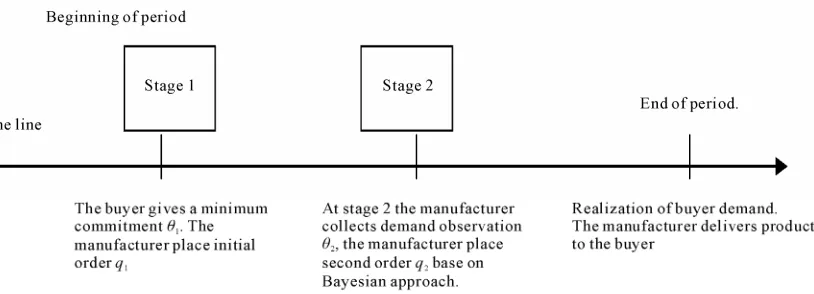
of X. The posterior distribution of X is defined by the observations of 1 and 2. Then manu-facturer places his second order quantity 2 if necessary. The time events of key component procurement process are shown in Figure 1.
q
We assume that the outputs are mainly limited by the available amounts of the key component, and the pro-duction cycle times are very short that can be neglected. After receiving the key components, the manufacturer produces the products immediately. Products are deliv-ered to the buyer at the end of period (immediately after second stage). Due to the demand uncertainty, the manu- facturer is difficult to determine two stage order quanti-ties.
In this paper we develop a two-stage dynamic optimi-zation model to decide the order quantity of a key com-ponent under a buyer’s minimum-commitment quantity contract. The model is formulated to maximize a manu-facturer’s profit. The following costs are considered in the model. 1) Key component unit cost: the unit cost of key component at stage 1 is and the unit cost at stage 2 is . 2) Holding cost: two kinds of inventories are considered. One is buyer responsible inventory, which only exists in the case of buyer’s real demand(x) below the minimum guaranteed quantity 1
(1) c (2)
C
Figure 1. Time events of key component procurement process.
and will be paid in the near future. The unit holding costs of buyer responsible inventory are the interest and in-surance. The other is manufacturer responsible inventory. The unit holding cost of manufacturer responsible in-ventory is the interest, insurance and obsolete costs. The holding costs of buyer responsible inventory and manu-facturer responsible inventory are h1 and ch2 respec-tively and h2 h1. 3) Shortage cost: two kinds of shortage cost are considered according to whether or not to pay shortage compensation. If the manufacturing out-put level is below
c c c
1
1, then there are two shortage types may occurred. The one includes general shortage cost and the compensation cost. The other is only the general shortage cost.The buyer’s minimum commitment and demand fore-cast updating in this paper belong to the category of minimum purchase commitment contract [1] and inven-tory management with demand forecast updates respec-tively [2]. Durango-Cohen and Yano [3] pointed out that increasing the level of commitment and information sharing will lead to the cost down of entire supply chain. Nowadays minimum commitment quantity contracts are commonly used in electronic industry. Anupindi and Bassok [1] classified the contract of quantity commit-ments and flexibility as three types. The first type is the total minimum quantity commitment contract. The sup-ply contract with total minimum quantity commitment is that a buyer gives his supplier a minimum ordering quantity commitment, and the supplier offers the buyer a discount price in return for the buyer’s commitment [4]. The second type is the total minimum dollar volume commitment contract. This contract is similar to the total minimum quantity commitment contract, but a buyer commits to a minimum business on the basis of dollar volume [5], and the supplier offers discounts based on the commitment of dollar volume. The third type is the periodical commitment with flexibility contract. Under such a contract, a buyer receives discounts for commit-ting to purchase in advance, and the buyer is allowed to
update his order amount in the rolling horizon basis. The rolling horizon flexibility (RHF) contract [6-8] is one kind of the third type. The RHF contract means the buyer has a “limited” flexibility to update his advance order after he commits to purchase certain quantity.
Gallego and Ozer [9] and Sethi et al. [2] classified the inventory information with demand updating problems as three types. The first type is the Bayesian analysis. This approach learns about further demand from the past history [10]. Dvoretzky et al. [11] first analyzed Bayesian models in the inventory problem. In this type, specific classes of demand distribution were discussed, such as exponential family of distribution [12], gamma family [13,14], negative binomial distribution [15], uniform- Pareto distribution [16] and normal distribution [17,18]. The second type is time-series models used in updating demand forecast, where they assume a correlation exists in the demand realization and construct the demand as a time-series model [10,19]. The third type is concerned with forecast revisions, such as Markovian forecast revi-sions model [20-22], single-period, two-stage ordering problem with demand forecast updating [23-26] and multiple period ordering problem with demand forecast updating [27,28]. A more comprehensive discussion can be found in [2].
Our study differs from the previous papers because we consider a shortage compensation policy for reducing demand uncertainty. Under the buyer’s minimum-com- mitment quantity contract and shortage compensation policy, two kinds of inventory and shortage costs are respectively formulated in the two-stage dynamic opti-mization model to decide the optimal order quantities.
some numerical examples, and sensitivity analyses of the major parameters of the model are performed. Finally, Section 4 concludes this article.
2. Problem Formulation
2.1. Notations 1
: buyer’s minimum-commitment quantity. 10
: shortage compensation range coefficient 0 1. [1,
1
1] is the shortage compensation range.(1
c ): unit ordering cost of key component at stage 1. (2)
C : unit ordering cost of key component at stage 2 is a random variable, and the corre- sponding probability
.(2) (2) (2) (2) 1 , 2 , , n
C c c c
{ , , , n}
P p p p (1) pc
1 2 : product unit selling price. . p
2
: the demand observation at stage 2. 1
h
c
c : unit holding cost of buyer responsible inventory. 2
h : unit holding cost of manufacturer responsible in-
ventory. 1 s
c : unit shortage compensation cost; cs10 2
s
c : unit general shortage cost; cs1cs20
X: buyer’s real demand, realization is denoted byx.
(1)
X : X(1) is a random variable to forecast the buyer’s demand at stage 1, (1)
1 X X . (2)
X : X(2) is a random variable to forecast the buyer’s demand at stage 2, (2)
1, 2 X X . 1(.)
f : probability density function (pdf) of X(1),
2 2
1, 0 1 X(1) N
2(.)
f : probability density function (pdf) of X(2),
(2) 2 2 2 2 2 2
1 2 0 1 0 1 0 1
2 2 2 2 2
0 1 0 0 1
,
X N
1(.)
F : cumulative density function (cdf) of. X(1) 2(.)
F : cumulative density function (cdf) of X(2). (.)
: standard normal probability density function. (.)
: the cumulative distribution function for standard normal distribution.
1(.)
(.)
: the standard linear loss function: : inverse function of (.). ( ) ( )d ( )
a
a x a
x .Decision variables: 1
q q
: order quantity at stage 1. q10 0 q 2: order quantity at stage 2. 2
Intermediate variables:
1: the decision space defined by 1
1q1q2 (1 )
(1 ) q q
. 2
: the decision space defined by 1 1 2.
11
q : optimal order quantity in 1 at stage 1
21
q : optimal order quantity in 1 at stage 2
12
q : optimal order quantity in 2 at stage 1
22
q : optimal order quantity in 2 at stage 2 1
q: optimal order quantity at stage 1 2
q: optimal order quantity at stage 2
2.2. Problem Assumptions and Formulation The mathematical model is formulated to determine the two stage ordering quantities of the key component for maximizing profit. The buyer’s real demand X is uncer-tain to be assumed following a normal distribution with an uncertain mean 0 and a given variance
2 0
, where 0
follows N(, 2 1
) with an unknown and a given variance 2
1
. At stage 1, after receiving the buyer’s minimum commitment quantity 1, the manufacturer uses 1 as an estimator of . The posterior distribu-tion of X after receiving 1 at stage 1 is denoted as
(1) 1
X X where
(1) 2 2
1 1, 0
X X N 1
(1) At stage 2, the marketing department collects informa-tion 2 about buyer’s real demand. We call it as an observation of X. The posterior distribution of X at stage 2 is denoted as (2)1, 2
X X where
(2) 2
1, 2 2, 2
X X N k
(2)
2 2 2 2 2 2
2 1 2 0 1 0 1 0 1
k (3)
2 2 2 2 2 2
2 0 1 0 0 1
(4) Because the manufacturer has the obligation to pro-vide the minimum-commitment quantity 1 to the buyer, the total order quantities q1q2 must be larger than 1. Now we will formulate the expected profit function and use a backward dynamic programming to determine the optimal q1 and q2.
We formulate the problem as a dynamic programming (DP) problem. For the DP formulation, the ordering times are given as the stages, stage 1 and stage 2. Deci-sion variable for stage n (n = 1, 2) is the ordering quan-tity n. The profit at the current stage depends upon the
current decision and the ordering quantity in the preceding stage
q
n
q 1 n
q . We set states for each stage n as
1 n
q .
With the backward solving procedure, first we should determine the optimal order quantity 2 at stage 2 in a given state 2
q 1
s q . We denote the expected profit func-tion at stage 2 as E(2)
q q2 1
. The state at stage 1 is known as s10. The expected profit function at stage 1 is denoted as E(1)
q1 , where
(1)
(1) 1 1 (2) 2 1
The optimal expected profit of the manufacturer is de-termined as follows:
lows:
1) Expected products sales
11
(1) 1 (1) 1
0
(1)
1 (2) 2 1
0 max max
q
q
E q E q
E c q E q q
(6) X
min ,
1 2
d2p x q q f x x
(9)2) Ordering costs when C(2)c(2)
where (2)
2
c q (10)
2
(2) 2 1 max0 (2) 2 1 q
E q q E q q
(7) 3) Expected holding costs:The unit holding cost of buyer responsible inventory is 1
h and holding cost of manufacturer responsible
in-ventory is . The holding costs can be expressed as follows:
c
2 h
c The items considered in E(2)
q q2 1
are expectedproduct sales, ordering costs, expected holding costs and expected shortage costs.
(2) 2 1 Expected revenues
Expected costs Expected product sales
Ordering costs Expected holding costs Expected shortage costs
E q q
(8)
1 1 2 1 2 1 1
2 1 2 1 1
for for
0 othe
h h
h
c x c q q x
c q q x x q q
2 rwise
(11) The expected holding costs can be formulated as fol-lows:
The relevant items are formulated respectively as fol-
h1 max 1 , 0 maxh2 1 2 1 , 0
2
dX
c x c q q x f
x x (12)4) Expected shortage costs:
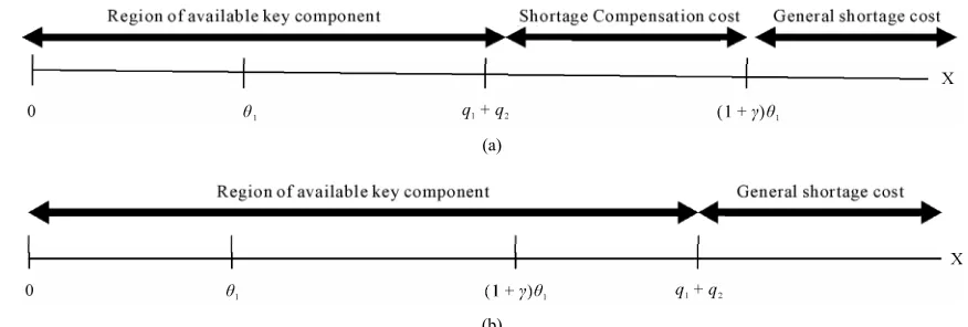
The decision space of total order quantity q1q2 can be divided into two subspaces 1 and 2, 1: total order quantity (q1q2) is less than
1
12 q q
, as shown in Figure 2(a); 2: total order quantity ( 1 ) is lar-ger than
1
1 , as shown in Figure 2(b). In 1, two kinds of shortage types may occur: 1) the shortage oc-curred between q1q2 and
1
1 belongs toshort-age compensation range, its unit shortshort-age costs are the shortage compensation cost and general shortage cost; 2) the others does not belong to shortage compensation range, its unit shortage cost is general shortage cost. The unit shortage costs of shortage compensation and general shortage are cs1 and cs2 respectively, cs1cs2. In 2, the shortage compensation cost does not occur. Two cases of shortage can be expressed as follows:
1 1 2 1 2
1 1 1 1 2 2 1 1
for 1 ,
expected shortage costs in 1 + 1 for 1 ,
0 ot
s
s s
c x q q q q x
c q q c x
1herwise.
x
(13)
2 1 2 1 1 2
2
for 1 ,
expected shortage costs in
0 otherwise.
s
c x q q q q x
(14)
Expected shortage cost can be combined as follows:
1 max min 1 1, 1 2 ,0 2max max 1 2 , 1 1 ,0 d
s s
c x q q c x q q
f2 x x (15)
(2) 2 1
E q q depend on the domain of the total order quantity q1q2,i.e., 1
1 2
1 1 2
1
2.3. Optimal Solution, 1
q q q q
and 1
q q1, 2
q1 q2
1
1
To solve the DP problem we first provide the optimal de- cisions for stage 2 under a given state s2q1. As men-tioned above the expected shortage costs in
, each domain
cor-responds to a shortage cost equation respectively (Figures (a) and (b)). Therefore E(2)
q q2 1
is formulated [image:4.595.67.540.502.616.2]
(a)
(b)
Figure 2. (a) in 1: total order quantity q1 + q2 is less than
1
1; (b) in 2: total order quantity q1 + q2 is larger than
1
1.for each domain as follows:
1 1 2 1
1 2 1
1 1 2
1 1 2
1
1
1 2 1
(2) 2 1 , 1 2 2 1 2 2 1 1 2
2 1 2 1 2 2 1 2 2
1
(2)
1 1 2 2 2 1 2 2
1
d ( )d d
d d
d 1 d
q q
h q q
q q q q
h h
s s
q q
E q q p f x x pxf x x p q q f x x c x f x
c q q f x x c q q x f x x
c x q q f x x c x f x x c q
dx
(16)
and
1 1 2 1
1 2 2
1 1 2
1 1 2
1
1 2
(2) 2 1 , 1 2 2 1 2 2 1 1 2
2 1 2 1 2 2 1 2 2
(2)
2 1 2 2 2
d ( )d d
d d
d
q q
h q q
q q q q
h h
s q q
E q q p f x x pxf x x p q q f x x c x f x
c q q f x x c q q x f x x
c x q q f x x c q
dx
(17)
We will show
1 2 1
(2) 2 1 q q,
E q q and
1 2 2
(2) 2 1 q q,
E q q
are both concave functions.
Then we can determine the optimal in the interval for the two cases respectively.
2 q
[0, )
Proposition 1. If and
hold for , then
1 2 0
s h
pc c pcs2ch20
2 [0, )
q
1 2 1
1 q q, q (2) 2
E q
and
2
1 2
(2) 2 1 q q,
E q q are concave functions, i.e.,
1 2, 1 0
q q
2
(2) 2 1 2 2
d E q q
dq
and
1 2 2
2
(2) 2 1 ,
2 2
0
q q
d E q q
dq
for q2[0, ) . Proof. See appendix A.
Proposition 2. Maximizing
1 2 1
(2) 2 1 q q, E q q
and
1 2 2
(2) 2 1 ,
q q
E q q
with respect to q2, we can get the optimal order quantity q2 denoted as q21
and
22
q for the two domains respectively as follows:
2 2 1
2 0 2 1 1
2 2 1
1 2 0 2 1
1 1 21
2 2 1
2 0 2 1 1
1 1
2 2 1
2 0 2 1 1
max 0,
if 1
max 0, 1
if 1
max 0, if
k t q
k t
q q
k t
q
k t
1
,
where
(2)
1 s1 2 1 1 h2
[image:5.595.75.513.79.227.2]
1 12 2 1
1 2 0 2 2
22 2 2 1
2 0 2 2 1
2 2 1
2 0 2 2 1
max 0, 1
if 1
max 0,
if 1
q
k t
q
k t q
k t 1 , where
(2)
2 s2 h2
t pc c pc cs2 (19)
Proof: See appendix B.
Then we provide the optimal solution for stage 1. At stage 1, the profit functions
1 2 1
1 2 1
(1)
1 ( ,q q) 1 (2) 21 1 ,
q q
q c q E q q
and
1 2 2
1 2 2
(1)
1 ( ,q q) 1 (2) 22 1 ,
q q
q c q E q q
correspond to 1 and 2 respectively. Due to 2 and being uncertain, the sample space of is
k ) (2)
C C(2
(2) ) (2 (2) 1 2 ,cn
,
p (2 C c
1 2
{ ,
P p
)
,c , ,pn}
with respect to the probability
, and the distribution of k2 is
4 2 2
1, 1 0 1
N . Let
1 2 1
1 2 1
(1) 1 ( , )
(1)
1 (2) 21 1 ( , ) q q
q q
E q
E c q E q q
and
1 2 2
1 2 2
(1) 1 ( , )
(1)
1 (2) 22 1 ( , ) q q
q q
E q
E c q E q q
be the expectation of
1 2 1
1 ( , )q q
q
and
q1 ( , )q q1 22 respectively, that are formulated as fol-lows:
1
1 1 3 1
2
1 2 1
1 2 1
1 2
1 2 1
1 1 3 1
( )
(1) 1 ( , ) (2) 2 1 , 2 2
1
(1)
(2) 2 1 , 2 2 1
( )
0, d
0, d
n q d d t
i q q K
q q i
K q q q d d t
E q p E q q f k k
E q q f k k c
q(20)
1 1 3 2
2
1 2 2
1 2 2
1 1 2 2 2
1 1 3 2
( )
(1) 2 1 ( , ) (2) 2 1 , 2 2
1
(1)
(2) 2 1 , 2 2 1
( )
0, d
0, d
q d d t
i q q K
q q i
K q q
q d d t
E q p E q q f k k
E q q f k k c
1 n q (21) where
1 2 1
2 2 2 2
(2) 2 1 , 1 2 0 2 1 2 0 2
2 2 1
2 1 0 2 1
2 2 2 2
1 2 0 2 1 2 0 2
2 2
1 2 1 1 2 0 2 1
(2) 2 2
1 2 1 1 2 0 2 2
(2) 0, 1 1 1 1 1 h h q q h s s s
h h s
h h s
h
E q q p c c k
p c c t
c c k
p c c c k
c c c c k k
c c
2 2 2 2 1
2 1 1 2 0 2 0 2 1
2 2 (2)
1 1 1 2 0 2 1
1 1
1 1 ,
s
s
c k
c k c q
t (22)
1 (2)1 s 2 1 1 h2 s1
1 2 1
2 2 2 2
(2) 2 1 , 2 1 0 2 1 2 0 2
2 2 2 2
1 2 0 2 1 2 0 2
2 2 2 2
1 2 0 2 1 2 0 2
2 2
1 2 1 1 2 0 2
2 2
2 1 1 2 0 2 1
1
0,
1
1 1
1 1
1 1
h s
q q
h h
s s
h h s
h s
s
E q q p c c q k
p c c k
c c k
p c c c k
c c k q
c
1
2 2
1 k2 0 2 1 ch1 2,
k
(23)
1 2 2
2 2 2 2
(2) 2 1 , 1 2 0 2 1 2 0 2
2 2 1
2 2 0 2 2 1 2 1
(2) (2) 2 2 1 (2)
1 2 2 2 0 2 2 1
(2)
2 2 2 2
0,
,
h h q q
h s h h
h h h
s h s
E q q p c c k
p c c t p c c
c c c k c c t c q
t p c c p c c
(24)
1 2 2
2 2 2 2
(2) 2 1 , 2 2 0 2 1 2 0 2
2 2 2 2
1 2 0 2 1 2 0 2
1 2 1 1 2 2 1
0,
.
h s q q
h h
h h h h
E q q p c c q k
p c c k
p c c c k c q
(25)
Proof: See appendix C.
We will show
and1 2 1
(1) 1 q q, E q
1 2 2
(1) 1 q q,
E q are both concave functions. Then we can search for optimal ordering quantity for each domain, expressed as (q11, q21) and ( , )
respec-tively.
12 q q22
Proposition 3. If pcs1ch20 and pcs2ch20 hold forq1 [0, ), then
and1 2 1
(1) 1 q q, E q
1 2
1 q q,
E q
2
(1) are concave functions of q1. where
1 2 1
2 2 2 1
(1) 1 , 1 0 2 1 2
1 2 4
2
1
1 1
n q q
i s h
i
E q q t
p p c c B
q B
B (26)
1 2 2
2 2 2 1
(1) 1 , 1 0 2 2 2
2 2 4
2
1
1 1
n q q
i s h
i
E q q t
p p c c B
q B
B
(27)
4 2 2
1 2 0
1 4 4 2 2 2
1 1 0 2 0
,
B
4 2 2 2
1 1 1 1 0 2 0
2 4 2 2 2 2
1 1 0 1 0
, q
B
2
4 2 2 2 2 2 2
1 1 1 1 0 2 0
3 4 2 2 2 2
1 1 0 2 0
, q
B
2
2 3 1
2 2
2
1 0 1
4 2 2 2
1 2 0
. 2π
B B B
B
B e
Proposition 4. If c(2)c(1)0 where
(2) (2)
1 i i i , n
c
pc i1, , n0
, then at stage 1 the optimal order quantity q11
and .
12 0 q Proof: See appendix D.
Proposition 5. There exists an optimal ordering quan-tity for each domain respectively, and the optimal order-ing quantity (q11
,
21
by the following procedure:
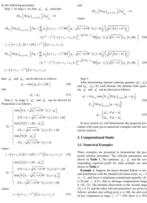
Step 1: At stage 1, we find q11 , q12 such that
1 2 111
(1) 1 q q, 1 0
q
E q q
and
1 2 2
12
(1) 1 q q, 1 0
q
E q q
, where
1 2 1
1
1 1 3 1
2
2
(2) 2 2 1 4 2 2
(1) 1 , 1 1 1 0 2 1 1 1 0 1
1
( )
(2) (1) 2 2
1 2 1 2 0 2 2 2
(2)
1 1 1 2 1
d 1 , n i s q q i
q d d t
s h K
s x h s
E q q p p c c q t
c c p c c q k f k k
t p c F c p c c
(28)
1 2 2
1
1 1 3 2
2
(2) 2 2 1 4 2 2
(1) 1 , 1 2 1 0 2 2 1 1 0 1
1
( )
(2) (1) 2 2
2 2 1 2 0 2 2 2
(2)
2 2 2 2
d
n
i s
q q
i
q d d t
s h K
s h s
E q q p p c c q t
c c p c c q k f k k
t p c c p c c
(29)then q11 and q12 can be derived as follows:
11 min 11, 1 1
q q (30) and
12 12
q q (31) Step 2: At stage 2, and can be derived by Proposition 2 as follows: 21
q q22
2 2 1
2 0 2 1 11
2 2 1
1 2 0 2 1
1 11 21
2 2 1
2 0 2 1 1
1 11
2 2 1
2 0 2 1 1
max 0,
if 1
max 0, 1
if 1
max 0, if
k t q
k t q q k t q k t 1 , where
(2)
1 s1 2 1 1 2
t pc F c pch cs1 . (32)
1 122 2 1
1 2 0 2 2 1
22 2 2 1
2 0 2 2 12
2 2 1
2 0 2 2 1
max 0, 1
if 1
max 0,
if 1
q
k t
q
k t q
k t
, where
(2)
2 s2 h2
t pc c pc c
Step 3:
After determining optimal ordering quantity (q11, q21) and (q12 , q22) for each domain, the optimal order quan-tity q1 and q2 can be derived as follows:
1 1 1
1 2
1 (1) 1 1
(1) 1 1 12
max ,
q q
q
q Arg E q q q
E q q q
11 (34)
21 1 11
2
22 1 12
, if , if
q q q
q
q q q
(35)
In next section we will demonstrate the proposed pro-cedure with some given numerical examples and the sen-sitivity analysis.
3. Computational Study
3.1. Numerical Examples
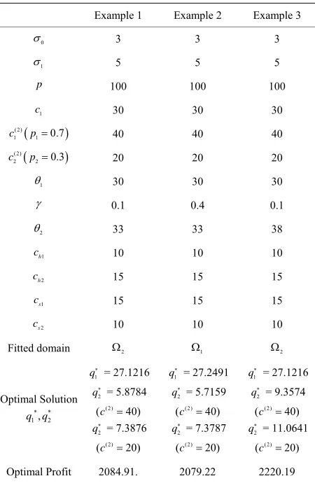
Three examples are presented to demonstrate the pro-posed solution procedure. The relevant parameters are shown in Table 1. The optimum 1, 2 and the cor-responding expected profit for each example are also shown in Table 1.
q q
Example 1. Suppose the buyer demand follows a nor-mal distribution with the standard deviation terms 03,
1 5
, and buyer’s minimum-commitment quantity (1) is 30 and is 0.1, that is, shortage compensation range is (30, 33). The demand observation at the second stage (2) is 33, and the other relevant parameters are given as follows: product unit selling price p is 100, the unit cost of key component at stage 1, (1)= $30, there is a 70%
c 2
[image:8.595.52.539.68.739.2]Table 1. Examples.
Example 1 Example 2 Example 3
0
3 3 3
1
5 5 5
p 100 100 100
1
c 30 30 30
(2) 1 1 0.7
c p 40 40 40
(2)
2 2 0.3
c p 20 20 20
1
30 30 30
0.1 0.4 0.1
2
33 33 38
1
h
c 10 10 10
2
h
c 15 15 15
1
s
c 15 15 15
2
s
c 10 10 10
Fitted domain 2 1 2
Optimal Solution
* *
1, 2
q q
1
q
= 27.1216
2 = 5.8784
q
( (2) 40)
c
2 = 7.3876
q
( (2) 20)
c
1
q = 27.2491
2
q = 5.7159 ( (2) 40)
c
2
q = 7.3787
( (2) 20)
c
1
q
= 27.1216
2 = 9.3574
q
( (2) 40
c )
2 = 11.0641
q
( (2) 20
c )
Optimal Profit 2084.91. 2079.22 2220.19
chance that the ordering cost at stage 2 will 40 and a 30% that the ordering cost at stage 2 is 20 ( (2)
1 40
c , 1 , , 2 ), per unit holding cost of buyer responsible inventory ( h1) = $10, per unit holding cost of manufacturer responsible inventory ( h2) = $15, per unit shortage compensation cost (
0.7
p c2(2)20 p 0.3 c
c
1 s
c ) = $15 and per unit general shortage cost (cs2) = $10.
With the proposed solution procedure, in step 1 we find that q11 27.3127 and q12 27.1216, then
11 min 27.3127, 1 1 33 27.3127
q
and q12 27.1216. In step 2, if c1(2)40 at stage 2,
2 2 1
1 2 0 2 1
1
30 32.4876
1 33
k t
and
2 2 1
2 0 2 2
1
30 32.8025
1 33
k t
,
then
21 max 0, 32.4876 27.3127 5.1749
q
and
22 max 0, 33 27.1216 5.8784
q .
If (2)
2 20
c at stage 2,
2 2 1
1 2 0 2 1
1 33 k t 34.0793
and
2 2 1
1 2 0 2 2
1 33 k t 34.5092 , then
21 max 0, 33 27.3127 5.6873
q
and
22 max 0, 34.5092 27.1216 7.3876
q .
In step 3, we get
1 1 1
1 2
1
1 (1) 1 1
(1) 1 1 12
max ,
max 2081.85, 2084.91 27.1216,
q q
q
q
q Arg E q q q
E q q q
Arg
11
2 5.8784 (if
q c1(2)40) or q2 7.3876 (if c2(2)20) and optimal expected profit is 2084.91.
Example 2. In example 1 the value of is changed from 0.1 to 0.4 while other parameters remain unchanged. With the proposed solution procedure, in step 1 we find that q11 = 27.2491 and q12 = 27.1216, then
11 min 27.2491, 1 1 42 27.2491
q
and q12 = 27.1216. In step 2, if at stage 2,
(2)
1 40
c
2 2 1
1 2 0 2 1
1
30 32.965
1 42
k t
and
2 2 1
2 0 2 2
1
30 32.8025
1 42
k t
,
then
21 max 0, 32.965 27.2491 5.7159
q
and
22 max 0, 42 27.1216 14.8784
q .
If (2)
2 20
2 2 1
1 2 0 2 1
1
30 ( ) 34.6278
1 42
k t
and
2 2 1
2 0 2 2 1
34.5092k t 1 42
,then
21 max 0, 34.6278 27.2491 7.3787
q
and
22 max 0, 42 27.1216 14.8784
q .
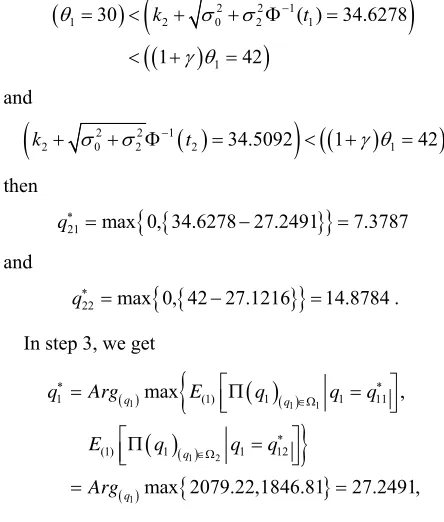
In step 3, we get
1 1 1
1 2
1
1 (1) 1 1
(1) 1 1 12
max ,
max 2079.22,1846.81 27.2491,
q q
q
q
q Arg E q q q
E q q q
Arg
11
2 5.7159 (if ) or 2 (if
q c1(2)40 q7.3787 c2(2)20)
and optimal expected profit is 2079.22.
Example 3. In example 1 the value of 2 is changed from 33 to 38 while other parameters remain unchanged. With the proposed solution procedure, in step 1 we find that q11 = 27.4702 and q12 = 27.1216, then
11 min 27.4702, 1 1 42 27.4702 q
and q12 = 27.1216. In step 2, if c1(2)40 at stage 2,
2 2 1
1 2 0 2 1
1 33 k t 35.7675
and
2 2 1
1 2 0 2 2
1 33 k t 36.479 ,
then
21 max 0, 33 27.4702 5.5298
q
and
22 max 0, 36.479 27.1216 9.3574
q .
If (2) at stage 2,
2 20
c
2 2 1
1 2 0 2 1
1 33 k t 37.3228
and
2 2 1
1 2 0 2 2
1 33 k t 38.1857 ,
then
21 max 0, 33 27.4702 5.5298
q
and
22 max 0, 38.1857 27.1216 11.0641
q .
In step 3, we get
1 1 1
1 2
1
1 (1) 1 1
(1) 1 1 12
max ,
max 2131.75, 2220.19 27.1216,
q q
q
q
q Arg E q q q
E q q q
Arg
11
2 9.3574 (if
q c1(2)40) or 11.0641 (if c2(2)20) and optimal expected profit is 2220.19.
3.2. Sensitivity Analysis 2
is an observation of
2 2 1, 0 1N
at stage 2. At stage 1 we don’t know what value of 2 will be ob-served. With Monte Carlo method we randomly generate 100 values of 2 from
2 2
1, 0 1
N , denoted as 2( )
i
, 1, ,100.
i ( ) 1
i
q
With the proposed solution procedure, we can find with respect to ( )
2
i
. Then we evaluate the average expected profit value for using in 100 val-ues of
( ) 1
i
q ( )
2
i
. The steps of Monte Carlo method are stated as follows:
Step 1: Randomly generate ( ) 2
i
, i1, ,100 from
2 2
1, 0 1 N .
Step 2: With each ( ) 2
i
we can find by Proposi-tion 5,
( ) 1
i
q 1, ,100
i respectively.
Step 3: Compute the expected profit values for using ( )
1 i
q in each 2( )i 1, ,100
i , denoted as (1)
q1( )i , ,
) ( ) 1i q (100
(excluding 2, parameters are fixed in
( ) 1 i iq i
( ) , 1, ,100 ). Let
* (1) ( ) (2) ( ) (100) ( )
( ) 1 1 1 100,
1, ,100.
i i i
i q q q
i
Step 4: optimal profit and optimal order quantity q1 can be derived as follows:
( )
1
* * *
1 q i max (1), (2), , (100)
q Arg .
The relationships among optimal expected profit, short- age compensation range coefficient ( ), and buyer’s minimum-commitment quantity (1) are shown in Table 1 with the related parameters given in the illustrating example. And the relationships among optimal expected profit, shortage compensation range coefficient () and shortage compensation cost cs1, are shown in Table 2 and Table 3.
[image:10.595.55.277.83.344.2]Table 2. Relationships among optimal expected profit, short- age compensation coefficient and buyer’s minimum-com- mitment quantity.
1
20 25 30 35 40
0 1836.02 2074.59 2345.81 2653.83 2990.32 0.1 1836.02 2074.59 2345.81 2653.83 2990.32 0.2 1836.02 2074.59 2345.81 2653.83 2990.32 0.3 1836.02 2074.59 2345.81 2653.83 2990.32 0.4 1836.02 2074.59 2345.81 2648.21 2985.97 0.5 1836.02 2067.19 2337.45 2645.42 2982.73 0.6 1832.17 2064.98 2335.56 2643.19 2980.85 0.7 1829.75 2064.86 2335.53 2643.11 2980.44 0.8 1829.53 2064.67 2335.47 2643.1 2980.41 0.9 1829.49 2064.65 2335.47 2643.1 2980.39 1 1829.48 2064.65 2335.45 2643.1 2980.39
Table 3. Relationships among optimal expected profit, short- age compensation coefficient and unit shortage compensa-tion cost (cs1) (given 1 = 30).
1
s
c
15 30 45 60 75
0 2345.81 2345.81 2345.81 2345.81 2345.81 0.1 2345.81 2345.81 2345.81 2345.81 2345.81 0.2 2345.81 2345.81 2345.81 2345.81 2345.81 0.3 2345.81 2345.81 2345.81 2345.81 2345.81 0.4 2345.81 2345.81 2345.81 2345.81 2345.81 0.5 2337.45 2321.75 2312.85 2299.03 2270.26 0.6 2335.56 2315.03 2301.06 2283.1 2264.03 0.7 2335.53 2303.37 2290.98 2270.67 2243.73 0.8 2335.47 2302.57 2287.84 2266.5 2229.04 0.9 2335.47 2302.48 2286.71 2260.49 2228.85 1 2335.45 2302.47 2286.7 2260.49 2228.84
1
, that is, when 1, the optimal expected profit is kept unchanged, but when 1, the optimal expected profit decreases accordingly, i.e., 20 = 0.5, 25 = 30 = 0.4, 35 = 40 = 0.3. The larger 1 is, the smaller 1 is. 2) The marginal optimal expected profit is increased as 1 increases. In Table 3, Table 4 and Figure 3 with a given 1 we find that when 1 (30 = 0.4, 40 = 0.3), the optimal total order quantity q1q2 is over
1
1 which causes the shortage compensation costcan not be occurred. Hence, if 40 then the manu-facturer can give the buyer a larger shortage compensa-tion value of cs1 and take buyer’s increasing the value of 1. For example, if the original shortage compensation coefficient = 0.2 and 1 = 30, then we find 30 = 0.4, the manufacturer can give = 0.3 and an arbitrarily large value of compensation cost cs1 to the buyer and take the buyer increasing the value of 1 from 30 to 40, then the optimal expected profit in the case of = 0.3 and 1 = 40 will be larger than it in the case of = 0.2 and 1 = 30.
Base on the above description, the management in-sights observed from Table 2 to Table 4 can be con-cluded as follows:
1) The more the buyer’s minimum-commitment quan-tity 1 is, the more the expected profit of manufacturer is.
2) There are some ways to induce the buyer to in-crease the value of 1:
a) From Table 2, we know the upper bound of (1) which the manufacturer can give to the buyer to attract the buyer increasing the minimum commitment value of
1
without losing the expected profit.
b) If the optimal total order quantity 1 2 is larger than
qq
1
1, then the manufacturer can give attractive values of shortage compensation cost cs1 (Tables 3 and4) and shortage compensation coefficient () (Table 2 to Table 4 to take buyer increasing the value of 1.
The manufacturer can provide alternatives for the buyer as Table 5 to induce the buyer to increase the value of 1.
Table 4. Relationships among optimal expected profit, short- age compensation coefficient and unit shortage compensa-tion cost (cs1) (given 1 = 40).
1
s
c
15 30 45 60 75
0 2990.32 2990.32 2990.32 2990.32 2990.32 0.1 2990.32 2990.32 2990.32 2990.32 2990.32 0.2 2990.32 2990.32 2990.32 2990.32 2990.32 0.3 2990.32 2990.32 2990.32 2990.32 2990.32 0.4 2985.97 2963.11 2940.85 2934.03 2930.33 0.5 2982.73 2956.39 2932.06 2909.27 2887.73 0.6 2980.85 2952.73 2926.98 2903.1 2880.74 0.7 2980.44 2951.93 2925.84 2901.67 2879.04 0.8 2980.41 2951.84 2925.71 2901.5 2878.85 0.9 2980.39 2951.83 2925.7 2901.49 2878.84 1 2980.39 2951.83 2925.7 2901.49 2878.84