Calibrating OD matrices with public transport and mobile phone data

(1)

Calibrating

OD-Matrices with

Public Transport and

Mobile Phone data

(2)

Documentation Page

Title Calibrating OD-Matrices with Public Transport and Mobile Phone data

Master thesis

Author B. Rorije

University of Twente

Discrete Mathematics and Mathematical Programming [email protected]

Supervisors Dr. G.J. Still

University of Twente

Discrete Mathematics and Mathematical Programming

ir. M.P. Schilpzand Omnitrans International Deventer

Keywords OD matrix, calibration, public transport, mobile phones,

OV-Chipkaart, GSM, GPS.

(3)

Summary

In traffic modelling the displacements of people between different zones are modelled. These displacements are stored in an Origin-Destination matrix (OD matrix). These matrices are often based on survey data or on a mathematical model. To improve these matrices so that they approach reality they are calibrated with real life data. At the moment this is mainly done with traffic counts.

In this thesis two different sources of information are studied, to see in which way they can also be used for OD matrix calibration. These sources are information from the public transport, and information from mobile phones. For public transport information three different models were defined, based on either counts, stops and journeys. For mobile phone datasets an algorithm was design to convert the data to a route in the route network. These four models were then implemented in the OmniTRANS program, which resulted in some conclusions and recommendations.

Samenvatting

In verkeersmodelleringen worden de verplaatsingen van mensen tussen verschillende zones gemodelleerd. Deze verplaatsingen worden opgeslagen in een Herkomst-Bestemmings

ma-trix (HD mama-trix). Deze matrices zijn vaak gebaseerd op een enquˆete of op een wiskundig

model. Om deze matrices te verbeteren zodat ze beter de werkelijkheid benaderen worden ze gekalibreerd met actuele data. Op het moment is dit vooral gedaan met verkeerstellingen

(4)

Preface

This thesis is the final part of my masters study Applied Mathematics at the University of Twente. It is part of the chair of Discrete Mathematics and Mathematical Programming, and the practical part of the thesis was done at Omnitrans International in Deventer, the Netherlands.

With this thesis the end of my masters study has been reached, and I look back on a fun and interesting time here in Enschede. Aside from studying I have been active at several cultural societies, which taught me a whole lot.

For this thesis I would like to thank my two supervisors, Maarten Schilpzand and Georg Still. They helped me a lot during the course of this thesis, and gave good advice on the structure and contents of this report. I would also like to thank my colleagues at Omnitrans International. It was fun working there, and there was always time to answer my questions.

Ben Rorije

(5)

Notations

An overview of all variables and symbols as they are used in this report.

Standard variables in a Network:

C set of all centroids,|C| c

with centroids i, jPC

N set of all nodes,|N| n

with nodesp, qPN

A set of all links,|A| a

with linklPA

S set of all stops,|S| s

with stopsf, kPS

T set of all (public) transit lines,|T| t

with transit lineoPT

Variables used for Calibration:

g OD matrix

with OD valuegij Pg

ˆ

g starting matrix for OD matrix calibrations

I set of all OD pairs,tpi, jq |i, j PC, iju

R set of all restrictions

restrictionr PR

ˆ

A set of links for which a traffic count is known

v set of all flows

flowvaPv on linkaPA

ˆ

v set of all flows belonging to a count

flow ˆvaPv on linkaPAˆ

Pijr Load on the path between centroidsiand j that is used for restriction r

r Elasticity of restrictionr

Sl Screenline matrix belonging to link l

(10)

Variables used for Public Transport:

H is the matrix containing all OV-Chipkaart data;

Hpf, kq is the number of people going from stopf to stop k

N_fbefore is the set of stops coming before stop f, on any transit line

N_fafter is the set of stops coming after stopf, on any transit line

pathspi, jq is the collection of all transit paths between centroidsiand j

Pijp is the percentage of flow going over pathpPpathspi, jq

T Lpplq is the transit line attached to linkl, on pathp

Variables used for Mobile Phones:

Ni all nodes inside areai

G(V,E) Graph describing the network,

(with V the set of nodes and E the set of links)

AB The link between nodesAand B

depA, Bq The Euclidean distance between two pointsA andB

Qi A GPS point, consisting of a pair of coordinatespxi, yiq

Q1..T Set of points given by the GPS data

Qt The projection ofQon the linkAB

ptE1..Epu The path along linksE1 toEp (with Ei,Ei 1 sequent)

Phones on,vehicle the number of active phones in a car

NofOccupants the number of people in a car

Pct_{phones/person} the percentage of people that have a mobile phone

Pctphones on the percentage of mobile phones actually turned on

NCk the real number of cars traversing routek

NPk the number of phones traversing routek

Rk the set of traffic counts attached to routek

Cr the total value of countr

(11)

1.

Introduction

77 77 77 77 77

Before starting any project it is important to look at what the goal of the project is, and what will have to be done to reach that goal. In section 1.1 a small background of the problem will be given, in section 1.2 the main project will be discussed, with the two steps that will be taken. And in section 1.3 an overview will be given of the structure of this thesis.

1.1

Background

In the area of traffic modelling and planning the OD matrix takes an important place. An OD matrix shows how many displacements there are from one location to another, which is a vital part of any traffic or transportation model. Because OD matrices are so much in use it is also important to have matrices that are ‘up to date’, meaning that they should give an accurate representation of the actual world. Keeping OD matrices up to date is done by performing calibrations, altering the OD matrices with information from the actual world.

In current OD matrix calibrations most information is taken from ordinary traffic counts. This works fine if they are applied to an older version of the OD matrix, or a matrix generated by a mathematical model. But sometimes traffic counts just aren’t enough and extra information is needed. In recent years there have been two developments that might give this extra information.

1.1.1 Public Transport

(12)

1.1.2 Mobile Phones

In recent years the number of mobile phones has increased dramatically. Many people today are carrying a mobile phone with them at all times, to stay in touch with others. When a mobile phone is switched on, it is tracked by the mobile network, in case someone else tries to call that person. But that also means that the location of anyone with a mobile phone is (in theory) known. And the location of a person can, amongst other things, be used for OD matrix calibration.

1.1.3 Modelling

Both the data from the public transport and from mobile phones is more than just counts on a link. They both have information about (a part of) a whole route from one person. If the data from both sources is just converted to counts this information will be lost. Therefore part of the modelling process will consist of trying to include as much information as possible into the calibration.

With the data from mobile phones there is another aspect. Mobile phone data shows only a percentage of all displacements, as not everyone will have a mobile phone. Therefore it must be studied if perhaps the data is representative to the rest of the population. In which case the data can perhaps just be multiplied to get the full number of displacements, which would save a lot of work.

1.2

Main Project

The main subject of this thesis is to research if information from public transport and from mobile phones can be used for OD matrix calibration and, if so, in which way. This research can be divided into two steps: Modelling and Implementation. In both phases the subjects of public transport and mobile phones will be treated separately, though some research has to be done to see if there is perhaps some overlap between the two.

1.2.1 Modelling

(13)

1.2.2 Implementation

After the modelling phase is complete it is also important to check if the proposed models can be implemented and do in fact work. Therefore a proof-of-concept has to be build, a prototype of the proposed adjustments. Depending on the format of the data, it has to be converted before it can be used. After that the implementation should work on several test-cases, proving the added functionality and better results.

1.3

Structure of the Thesis

This thesis is build up into four parts. The first part, Part 0 consists of the literature research done at the start of the final project. In Chapter 2 the general part of the literature research is given. In Chapter 3 an introduction is given into the company for which this thesis was written, Omnitrans International, and their program, OmniTRANS. And in Chapter 4 some specification is given to the above problem description, based on all the information from the literature research.

After the literature research the two areas, public transport and mobile phones, are treated separately. In Part I the public transport is treated. For this area first some introduction is given in Chapter 5, together with the first steps into the modelling. Then in Chapter 6 some algorithms are defined and discussed, to help with the modelling of the public transport model. In Chapter 7 then three options are treated, that flow from the model and the different algorithms. Then in Chapter 8 the implementation of these three options is given, with a small overview of the encountered problems and their solutions. And finally in Chapter 9 some tests are discussed, together with the results gathered from these tests.

In Part II the modelling and implementation of the mobile phone area is discussed. In Chapter 10 first a small introduction is given, together with an outline of the needed steps to successfully model the mobile phone datasets. In Chapter 11 two algorithms are given to convert the mobile phone datasets into routes through the network. Then in Chapter 12 some steps are given into processing the routes, such that they can be used for OD matrix calibration. In Chapter 13 the implementation of one of the two algorithms is given, together with some adaptations made to the algorithm. And in Chapter 14 again some tests are done on the algorithm, and from these tests some results are given.

(14)

2.

Literature Review

77 77 77 77 77

In this chapter the results of the Literature Review will be given. In section 2.1 some general background information is provided as an introduction into the research area. In section 2.2 the calibration of OD matrices is treated, together with some solution methods. Then in section 2.3 an overview of public transport and the OV-Chipkaart is given, while section 2.4 contains a background of mobile phone data.

2.1

General Background

Transport Modelling is a very large field with a lot of different topics in it. Most models in transport modelling have to do with networks and the displacements in them, people or goods moving from one place to the other. This report will mainly focus on traffic modelling, the modelling of vehicles and persons in cities and/or other areas. And then especially on improving an existing model, by calibrating certain parts of the model.

2.1.1 Four-step Model for predicting traffic flows

In the area of traffic modelling the following Four-step model is often used [Ort´uzar &

Willumsen, 2001]. It has been around for more than fifty years, and lies at the basis of most transportation models used today.

The Four-step model assumes that a network of links is already known. First the area is di-vided into different zones, when the area is a city these zones are often modelled on the postal codes. All zones are connected to each other by the network of links (roads/tracks/other). These zones are then filled with socio-economic data, consisting of the number of residents in that zone, the number of jobs in that zone and any other attractions that are located in that zone (i.e. shopping centres, amusement parks, etc.). After adding the socio-economic data the following four steps are applied.

1. Trip generation

(15)

2. Trip distribution

After step 1 only departures and arrivals are known. In the second step these are connected, as a departure from one zone belongs to an arrival at another zone. These trips are then stored in an Origin-Destination matrix (OD matrix), defining the number of trips between each origin and destination. Linking the origins and destinations can be preformed by several different methods. Two methods often used are the Fratar model (also called Growth Factor model) and the Gravity model. The Gravity model will be treated in the next section.

3. Modal split

With all the trips known, it becomes important to look at the mode of each trip, i.e. what kind of transportation is used. The mode can be by car or public transport (trains, trams, buses, etc.), but other modes can also be used (for example cycling or walking). For every mode a separate OD matrix is created, only containing trips belonging to that specific mode.

4. Route Assignment

Now that every trip has an origin, a destination and a mode the exact route of the trip can be assigned. Route assignment is the most difficult step of the problem, as there are many things that have to be taken into account. For example some links have a maximum load, other links can only be used for one type of mode (highways for cars, train tracks for trains). Another difficult aspect is congestion: the route of a trip is dependent on congestion, but also influences it. This is why often an iterative approach is used, searching for a user equilibrium.

2.1.2 Gravity Model

The gravity model is based on the principles of gravity. Gravity says that two objects always attract each other, and that this attraction is based on the mass of the two objects,

m1 and m2, and the squared distance between them, r2. In formula the above can be

written as:

F Gm1m2 r2

For transport modelling the formula becomes:

Ai,j αPiPj

pdi,jq2

In the formula the trip goes from originito destinationj, withAi,j the attraction between

these two. Pi and Pj are the population sizes of zones iand j, respectively, anddi,j is the

distance between zonesiand j.

(16)

quicker than others, meaning that distance is perhaps not the best measure to use. Together this leads to:

Ai,j αOiDjfpi, jq

withOi the number of departures from origin i,Dj all arrivals at destinationj, andfpi, jq

a general measure of the travel cost between zonesiand j ([Ort´uzar & Willumsen, 2001]).

The implementation of the Gravity model into OmniTRANS can be found in section 3.4.

2.2

OD Matrix Calibration

Between steps 3 and 4 in the Four-step model another step is needed. Because the OD matrices from steps 2 and 3 are not based on ‘real’ results (they are mathematical models),

they are not guaranteed to have good results. Therefore the OD matrices have to be

calibrated to approximate the real world. There are several different methods that can be used to calibrate an OD matrix.

In the past OD matrices were calibrated with information that came from a whole range of surveys, everything from roadside interviews to home interviews and license plate tracking. But these methods are very expensive and time consuming, as a lot of information is needed to create a good OD matrix. Therefore researchers looked at other, more easily obtainable data, to use for creating a good OD matrix. Eventually they decided on using traffic counts. Traffic counts are easily obtainable, and are used in a wide variety of applications, which means that they are also widely available.

Note: In the literature sometimes the term “OD matrix estimation” appears. This term is more used to indicate that the OD matrix is created from the counts or surveys, and not changed (calibrated) by counts or surveys. Therefore the term OD matrix estimation really means something else, and is not applicable for this thesis.

2.2.1 Problem specification

Every origin and destination is located on a road network. A road network is build up from

a set of nodes, calledN, and the set of links between these nodes, called A. Traffic counts

are known for some links, the set of these links is called ˆA. On every link there is a flow of

traffic, the set of all flows is called v tva| aPAu. For the links in ˆA the flow is known

from traffic counts, the set of these flows is called ˆv tvˆa|aPAˆu.

Origin-Destination matrices contain all the possible pairings between an origin and a

des-tination. Define the OD matrix to be g, then the number of people going from origin i

to destinationj will be gij. Intrazonal trips are not taken into account, therefore gii 0.

Calibrating an OD matrix works with a ‘starting’ matrix, ˆg, derived from the Four-step

model. The starting matrix will be calibrated with the counts from ˆAto create the ‘target’

(17)

This gives rise to the following General Problem formulation (GP):

min

g,v Fpg,vq αF1pg,gˆq p1αqF2pv,vˆq

s.t. vassignpgq, (GP)

g¥0,

v¥0.

In the above descriptionF1 andF2are the distance measures betweengand ˆg, and between

v and ˆv, respectively. α is a constant on the interval r0,1s, and indicates the level of

confidence in the original matrix. Ifα is close to 1 the new OD matrix lies close to the old

OD matrix, ifα is close to 0 the new OD matrix is heavily influenced by the traffic counts.

The assignment of g, represented by v, is on its own also an optimization problem. v

is the solution of a route assignment, assigning the OD flows from g to routes on the

network, subject to the constraints on the road network, and thereforev is the solution of

a user equilibrium. This means that(GP)is a bi-level problem, in that there is interaction

between the constraints and the objective function. In each iteration a new route assignment

is made, changing the valuesvand therefore the influence of ˆv.

There are many methods and algorithms for the route assignment of g. In Chapter 3 two

methods for a route assignment will be treated, as part of the introduction into Omni-TRANS.

2.2.2 Solving methods

For solving the general problem above there are several methods. These methods can be divided into three areas: Minimizing Information, Statistically Interference and Gradient Based Solutions. In the next section they will be briefly treated, using information from [Abrahamsson, 1998] and [Spiess, 1990].

• Minimizing Information

The Minimizing Information approach works from the premise that the information from traffic counts will never uniquely define the target OD matrix. Therefore this method tries to minimize the amount of information that is added to the starting matrix in the calibration. That way the end result is an OD matrix, changed to include all the traffic counts, but still as close as possible to the starting matrix. The Minimizing Information method is sometimes also called the Entropy Maximizing approach, as minimizing information is the same as maximizing entropy.

• Statistically Inference

(18)

There are three main methods in the area of Statistically Inference:

- Maximum Likelihood, - Generalized Least Squares, - Bayesian Inference.

These three differ in the distribution that they use, and therefore also in their definition

of the objective functions F1 and F2.

• Gradient Based Solutions

With Gradient Based solutions the starting OD matrix is changed, in the ‘direction’ based on the gradient of the objective function. Every time a traffic count is added the objective function changes, and the algorithm will look in a new direction. Because the gradient is used for determining the optimal direction, this direction will always point to the largest yield.

The Gradient method is probably the most widely used algorithm today, and therefore it will be used in the rest of this report, together with OmniTRANS’ own algorithm. The specific Gradient algorithm that will be used will be the one from [Smits, 2010], which will be further explained in section 3.7.

2.3

Public Transport

Public Transport is the generic term for a lot of different types of transport. The fact that it is called ‘public’ comes from the fact that companies providing public transport are (partly) funded by the government. This fact also means that they are required to offer their services to everyone. Most public transport services are bound by a (strict) timetable.

2.3.1 PT Modes

As said before, there are a lot of different types of public transport. Public transport can be categorized in the following three ‘modes’ [Wikipedia, 2010]:

• Buses and Coaches

Buses and coaches are large car-like vehicles, operating on conventional roads. Both transport passengers from and to stops, which are often specially marked and placed along their route. They have a low capacity in comparison to track-based transport, and therefore are used mostly for short distances or for routes where there are no track-based alternatives.

• Track-based Transport

(19)

Track-based transport comes in three types:

- Trains

Trains transport passengers between cities, following a specific route along a series of cities, towns, villages and stations. Trains follow a strict timetable, as they are not influenced by normal congestion on the road network.

- Trams and Light rail

Trams are track-based vehicles that drive (at least partially) on the conventional roads, mixing in with the rest of the traffic. Trams are smaller than trains, and therefore also have a lower capacity. Light rail is a combination of a tram and a train, designed in such a way that it can both ride on tram tracks and train tracks.

- Rapid Transit

Rapid Transit is a generic name for both the Metro, Subway and the Underground. In general rapid transport is quicker than trams and buses, and has more capacity. The difference is that rapid transit is often based in the tunnels beneath a city, needing special entrances and exits.

• Ferry

Ferries are boats or ships transporting passengers and vehicles over water. In the case of public transport ferries are often small boats, used for transporting cars and pedestrians across a (small) river or channel. Some ferries have strict timetables, leaving at specific times, others will only depart if enough people are on board.

2.3.2 OV-Chipkaart

In recent years a lot of countries have adapted some sort of electronic travel ticket or card

for their public transport [Pelletieret al., 2009]. The appeal of electronic travel cards is easy

to see: it prohibits fare dodgers, gives companies insight in the travel habits of passengers and makes it easier for the passengers to pay for their tickets. This section will give an overview of the Dutch version of the electronic travel card, the “OV-Chipkaart”.

Background

(Most information in this section comes from [Ministry of Transport, Public Works and Water Management, 2008] and [OV-Chipkaart.nl, 2010])

(20)

At the moment there are two regions (Amsterdam and Rotterdam) where the OV-Chipkaart is the only valid payment method in the metro, tram and bus. In the provinces Groningen and Drenthe, and in trains run by local companies, the OV-Chipkaart had some delays, and for the moment cannot be used at all. In the rest of the country and in the trains of the NS a dual system is in place: both the OV-Chipkaart and the old payment options are valid.

The OV-Chipkaart has three different card types, which are differentiated by who will use them.

• Personal card

Personal cards are for people who travel a lot with the public transport, or who have a subscription to a specific route or discount (people over 65, students, etc.). They feature a photograph and some personal information about the holder, so it cannot be used by anyone else.

• Anonymous card

Anonymous cards are for people who travel only once in a while, or people who share their card with others. They do not feature any personal information, and are therefore also used by people who prefer not to share their personal information with the travel companies.

• Disposable card

Disposable cards are for people who rarely use the public transport, like tourists. After it has been used it can be disposed easily, as it cannot be recharged.

Not much is known about when the OV-Chipkaart will be the only valid payment method for the public transport in the Netherlands. The NS already reported that they will keep accepting paper tickets until the majority of passengers have switched to the OV-Chipkaart. There have also been some problem with transfers from one company to another: they some-times resulted in the passenger paying too much. Minister of Transport, Public Works and Water Management Eurlings responded that the full implementation of the OV-Chipkaart will be delayed until that issue is resolved [Minister C. Eurlings, 2010].

Data from the OV-Chipkaart

One of the reasons the OV-Chipkaart was introduced was for the information it gave to the public transport companies ([Ministry of Transport, Public Works and Water Management, 2008]). Before they introduced the OV-Chipkaart, they had to hold numerous surveys and counts just to get an idea of how many people used which services on which time.

(21)

In the area of OD matrix calibration there have been almost no publishings on how to use information from the public transport. Two studies that do use data from electronic travel cards, [Chan, 2007] and [Cui, 2006], only use it in a special model where only public transport is taken into account. No studies were found that actually used public transport data together with the regular traffic data in one model.

Information from electronic travel cards is however used for a wide variety of other studies. For example some companies are trying to find demographic groups for additional mar-keting. Other companies want to develop real-time information on conditions inside the network, in case additional personal or material is needed. There also have been several studies trying to find the precise path used by passengers (which is only useful in networks

where multiple routes are possible) [Pelletier et al., 2009].

2.4

Mobile Phones

Mobile phones are starting to become an integral part of our society. They give people the ability to call and be called, even when they are not at home or at work. They allow them to send short messages to each other, and even to surf the internet or make photographs. In recent years this has escalated with the introduction of so-called “smart phones”, mobile phones that offer much more in the way of processing power, connectivity and applications.

Mobile phones use special mobile communication networks. These networks are managed by a mobile operator, for example Vodafone or Orange. How the different networks function is based on the kind of system that is used. The largest mobile communication system that is in use today is the Global System for Mobile communications (GSM) network, and therefore for this thesis only that network will be considered.

Another aspect of mobile phones today is that some of them are carrying a Global Position System (GPS) locator with them. A GPS locator interfaces with satellites in the sky, giving the user the coordinates of his or her location. These locations are sometimes stored, and can be used for finding the exact route of that mobile phone. Therefore also GPS datasets will be considered in this thesis.

2.4.1 Global System for Mobile Communications

(22)

Background

The GSM system differs on several points from other systems. For one they use a so-called SIM (Subscriber Identity Module) card. These cards contain a unique identification number that identifies a user on the network, so that the network knows which user can be reached at which transceiver. Because this information is located on a card it can be removed from one mobile phone and inserted into another, giving more freedom to users. Other systems do not have this ability, and therefore users cannot easily switch between mobile phones.

GSM is also the system that introduced the term roaming to mobile communications. When someone is using a mobile phone that phone has a connection to a nearby transceiver. But if the person is travelling the mobile phone might leave the range of that transceiver, and enter the range of the next one. The GSM system then automatically hands the connection over to the next transceiver, allowing the mobile phone to ‘roam’ through the network. After the GSM system implemented roaming it was quickly duplicated by the other mobile phone systems.

Base Transceiver Stations

The GSM system works over a whole network of transceivers, spread across the world. Every transceiver is capable of accepting phone calls, text messages and, in recent years, internet connections. Transceivers are build up of ‘cells’, antenna’s with a certain range and capacity. Every cell can handle about 40 phone calls at one time, and in busy cities transceivers are equipped with multiple cells, just to offer enough service for everyone. There are five different types of transceiver cells, based on their range:

• Umbrella-cell (Very long range)

Umbrella-cells have the longest possible range found among transceivers, 35 kilometres. Umbrella-cells are often used for overlaying coverage, spanning the areas between two

other cells where coverage is at its lowest. They are also used for highways and

roads where people move at high speeds, when a lot of transitions between different transceivers are made. In that case the connection will be handed to the umbrella-cell, which will cause the number of transitions to go down dramatically.

• Macro-cell (Long range)

Macro-cells are often located in the countryside, where there is only a small demand for coverage and therefore a few cells can give enough coverage to a large area. Each macro-cell has a range of 2 to 10 kilometres, based on the surroundings of the cell.

• Micro-cell (Medium range)

(23)

• Pico-cell(Short range)

Pico-cells are small transceivers that are often put in places where the other transceivers cannot reach, for example in tunnels and large buildings. They are also used to increase coverage on a very busy point, like a train station. Pico-cells have a maximum range of 100 metres.

• Femto-cell (Tiny range)

Femto-cells are the newest addition to the set of transceivers. They are designed for offices and houses, to increase the coverage inside buildings. That is why femto-cells only have a range of about 10 metres, and can only handle 10 to 16 phones at one time (for residential homes this is 2 to 4 phones).

Data from the GSM network

Mobile phones that are active (but not calling/messaging) will regularly send out a signal, telling the network where it is. It does this by connecting to the nearest transceiver and transmitting their SIM code. That transceiver updates the SIM code into a Visitor Location Register (VLR). That way, if another phone tries to reach that phone it only has to check the VLR to see if the phone is in that specific location.

Through different operators different data is stored in the VLR, which means that GSM datasets often differ from each other. Sometimes so much information is stored that the exact location of a mobile phone can be traced, other times only a broad area is known where the mobile phone could have been.

The data from mobile phones is already used in some projects, though not for OD matrix calibration. A prime example is the agreement between TomTom and Vodafone. Voda-fone supplies TomTom with depersonalised information about their mobile phones, which TomTom uses in traffic modelling and congestion warnings.

2.4.2 Global Positioning System

GPS locators in mobile phones are a new ‘feature’, giving users the possibility to check their own location, and based on that location get recommendations for restaurants, public transport timetables and other useful information. But those locations are also stored in a database and can therefore be used for OD matrix calibration.

Background

(24)

As GPS was devised and constructed by the US military they were also the only ones able to use the system. This changed when in 1983 a Korean aeroplane flew into Russian airspace, due to navigation errors, and was consequently shot down. That event caused President Reagan to make GPS available for civilian use, when it was fully operational, in April 1995. Today the GPS system is still owned and operated by the US government, which reserves the right to deny the GPS service on a regional basis, in case of war and other conflicts.

GPS locators work by connecting with the satellites in orbit. Each satellite sends out a signal containing the time the message was transmitted, the precise orbital data of that satellite, and the status and orbit of all the other satellites. With data from several satellites the locator then calculates its own exact location.

Data from GPS locators

GPS locators take a certain amount of time to find their exact location. Because users might not want to wait, the locator keeps itself up-to-date, regularly checking its location. These updates are sometimes stored at the mobile phone provider, due to European and American law. These laws state that mobile communications providers have to be able to provide the exact location of their mobile phones in a certain amount of time. The reason for these laws is for the emergency numbers 112 and 911, when they are called the emergency service has to know where the caller is at that moment. That is why those restrictions were placed on mobile phone providers, and that is why they store GPS coordinates of their customers.

The GPS coordinates can be given in longitude and latitude, but that is not always the case. Sometimes the coordinates are given in another format, also called “datum”. These datums differ in the way the shape of the earth is modelled, and therefore how the round surface of the earth is converted to a 2-dimensional picture.

There are some projects that use GPS datasets for a variety of studies concerning traffic flows, decisions based on road-side information and modelling OD matrices. Most of these datasets however are generated by car navigation systems or specially placed GPS locators, and not with data from GPS locators in mobile phones.

2.4.3 Map Matching

(25)

There has been a lot of research done in the area of map matching with respect to GPS data

([Qudduset al., 2007]), but not really anything for GSM data. For some GSM datasets the

same methods can probably be used, but this is not the case in general. The real difference between GPS and GSM data is that the GPS datasets contain actual coordinates, while GSM datasets have areas where the mobile phone could have been. This difference will mean that both types will have to be modelled and implemented in a different way.

(26)

3.

Introduction to OmniTRANS

77 77 77 77 77 77 77

In this chapter the software OmniTRANS will be introduced. In section 3.1 some background information about OmniTRANS and its history will be given. Sec-tion 3.2 introduces the dimension as they are used in OmniTRANS. Then in sec-tion 3.3 the structure of a network is given. Secsec-tion 3.4 treats the trip distribusec-tion in OmniTRANS, with the implementation of the Gravity model. Section 3.5 will give two methods for the route assignment. Section 3.6 treats the calibration of OD matrices, and finally in section 3.7 the future gradient descend method will be given.

(Most information in this chapter comes from [Smits, 2010], [Omnitrans, 2010] and [OmniTRANS, 2010])

3.1

Background Information

According to their official site OmniTRANS is “Transport Planning Software” [Omnitrans International, 2010]. This means that it models “Transport” (displacements, people or goods moving from one location to another), then starts “Planning” (evaluating, assess-ing and (re)designassess-ing the network and data), combinassess-ing both Transport and Plannassess-ing in “Software” (a computer program).

OmniTRANS was originally designed and implemented by a company called Goudappel Coffeng, the largest Dutch Traffic and Transport consultancy. During the nineties Goudap-pel Coffeng noticed that the software that was in use for traffic and transport modelling was inadequate for their needs. Things that were unsatisfactory were for example a poor interface, lack of data management capabilities, limitations of the project sizes and the inability to (correctly) transfer model runs.

These limitations led to the decision to start the development of their own software, called OmniTRANS. The development of OmniTRANS took 9 months, and after it was offered to Goudappel Coffeng’s customers, who were at the time using other software, almost all of them decided to switch to OmniTRANS. Due to the positive response, Goudappel decided to continue developing OmniTRANS. In May 2003 the popularity of OmniTRANS convinced Goudappel to market OmniTRANS internationally, and therefore formed the company Omnitrans International.

(27)

the model. A third aspect is the ability to also work with dynamic models, working with different time intervals and even with predictions of trends. OmniTRANS also has a clear user interface, and for expert users has a whole range of classes and features to improve modelling and solving.

3.2

Dimensions

In every computer program data that is entered has to be first divided into categories, for the structure of the data. These categories are also called dimensions, as data is some-times entered as a hypercube (a multi-dimensional matrix), with the categories acting as dimensions. In OmniTRANS there are four standard dimensions; purpose, mode, time, and user-defined. For every trip that is generated in OmniTRANS these dimensions are given. Together the dimensions are often called PMTU, why will be explained after the dimensions themselves have been treated.

• Purpose

Purpose defines the objective of a trip. A purpose can be for example going ‘from home to work’, or going ‘from work to shopping’.

• Mode

Mode defines the type of transport. Two examples of modes are ‘car’ and ‘public

transport’.

• Time

Time is the time interval in which the trip takes place. A time interval can be for example just ‘from 10:00-10:15’, or the whole ‘AM peak’.

• User-defined

User-defined dimensions can be anything the user might want to implement. Examples of dimensions can be ‘car ownership’, or a differentiation of internal/external traffic.

Aside from these four dimensions another two dimensions appear in OmniTRANS, at the moment OmniTRANS has generated its own data. These two dimensions are:

• Result

Result is the solution after OmniTRANS has finished a certain number of iterations in an algorithm, for instance a route assignment or an OD matrix calibration.

• Iteration

Iteration is the current step in the calculations.

(28)

3.3

Modelling a Network

Before OmniTRANS can do any calculations a network has to be modelled. For the network first a map of the area is entered in OmniTRANS. This area is then divided into zones, and at the centre of each zone there is a centroid, a representative point of that zone. Each centroid has information about that zone, like the number or residents and jobs. Additional centroids are added for “the rest of the world”, so that traffic that enters/leaves the area can also be modelled.

Centroids are connected to the road network, which is represented by nodes and links. Every road is represented by a link, a line in the network. Every link has certain properties like capacity, length and type (which mode of vehicle can use that link). In most models every link has a distinct direction, which means that two way streets have to be modelled by two links. But in OmniTRANS these are modelled by one link, with two sides that can be defined separately. Not all roads in a network will be represented by a link, small residential streets and dead-end streets will often be skipped.

[image:28.595.83.515.429.713.2]

At every point where two or more links meet a node is placed, connecting the links together. Nodes are mostly used as junctions (if there are more then two links attached), though not every junction in an area is modelled. As with real junctions there are several characteristics that influence the travel time, for example the approaching lanes (separate lanes for turning left/right), and the presence of traffic lights. These characteristics have an effect on the flow and speed of traffic and therefore have to be included in the model.

(29)

3.4

Trip Distribution

Trip distribution is the process of linking origins and destinations together, to create trips. Trip Distribution is often done with a mathematical algorithm. In OmniTRANS the Gravity model is used, and therefore the implementation of that model into OmniTRANS will be discussed in this section.

In OmniTRANS there is a whole class of procedures for solving the gravity model: Ot-Gravity. The OtGravity class first calculates the “production” and “attraction” of every centroid, based on the total number of trips leaving/arriving at any other centroid. But that means that only separate departures and arrivals are known. The goal is then to distribute these trips such that departures and arrivals are linked together.

OtGravity does the trip distribution with a doubly constrained model. On one hand it will balance the trips between each zone to the travel cost between the two zones. And on the other hand it will try to keep as close as possible to the original constraints created by the productions and attractions of each zone. OtGravity does this with an iterative approach, hopefully converging to a good solution. Because the productions and attractions are often not in balance (if there are in total more people leaving than arriving, or the other way around) there is also the option to either use only the attractions or only the productions.

The travel cost between two zones can be influenced greatly by the user. The travel cost can be dependent on time, distance, number of junctions, or any other generalized cost. Aside from the travel cost also the “perseverance” of travellers is needed. The perseverance will tell OtGravity how much cost the travellers are willing to ‘pay’ to get to their destination. With the measure of perseverance OtGravity will be able to distribute trips over the different zones, with a distribution function. There are at the moment four functions implemented in OtGravity:

Log-normal Fvpzijvq αvepβvln

2_p_z

ijv 1qq

Top Log-normal Fvpzijvq αvepβvlnpzijv{γvqq

Exponential Fvpzijvq αvepβvzijvq

Defined by a discrete array rrx1, x2, .., xns,ry1, y2, .., ynss

In the above formulas Fv is the distribution function for mode v, zijv is the impedance

(travel cost) between centroidsiand j for modev, and α,β andγ are parameters.

3.5

Route Assignment

As mentioned in Chapter 2 two methods for the assignment of traffic flows from the OD

matrix will now be discussed. A reminder: the “assignment of g” is distributing the trips

over the network, finding a path for every trip. The assignment of g not only influences

(30)

3.5.1 All or Nothing (AON)

All or Nothing is the simplest route assignment possible. First the shortest path between every zone is calculated, there are several different algorithms that do that. In OmniTRANS a reverse propagation algorithm is used, starting at a destination and working backwards until it has reached every other zone. After the shortest paths have been found the as-signment is simple: just sent all traffic across that path. Therefore an AON asas-signment is actually the first step in a ‘normal’ user equilibrium computation.

Of course there are two very big downsides to the AON approach. The first downside is that it can happen that the assignment through the network can exceed the capacity of one or more links in the network. This is of course impossible in practice. The second downside is that an AON assignment doesn’t take congestion into account. This means that, even if the capacity is not exceeded, the travel time can go up, just because there are too many vehicles on the road. And therefore trips will actually use a different route, avoiding the congestion.

Despite these two downsides the AON assignment can give good results in small networks where congestion isn’t a problem. It is also very useful to give a first impression of a network, to see if it is going to be congested or not (exceeding capacities is a good indication of congestion).

3.5.2 Volume Averaging (VA)

Volume averaging is a little bit more complex compared to AON, but it gives much better results. VA works with volumes, which is just the amount of traffic flow on a link. The assignment itself is done with an iterative process: the volume in one iteration is dependent on the volume from the last iteration. In the first iteration the volumes found by an AON assignment are used, for the other iterations the following formula is used:

V_ln p1φqV_ln1 φFl p0¤φ¤1q

withVn

l the volume on linklin iteration n,Fl the volume on linkl from the AON

assign-ment, andφ indicating how close the solution should stay to the AON assignment. φcan

be a constant or change depending on the number of iterations.

3.5.3 Travel Time Functions

(31)

The BPR-function works with the following formula:

TlTl0

1 αpVl{Qlqβ

whereTl is the travel time on linkl,Tl0 is the travel time without the effects of congestion,

Vl and Ql are the volume and capacity of linkl, respectively, and α and β are parameters

of the model.

3.6

OD Matrix Calibration

For the calibration of OD matrices OmniTRANS has created a specific class: OtMatrix-Estimation. The OtMatrixEstimation class contains several techniques that can help with calibrating the OD matrix. In the process of calibrating in OmniTRANS also other in-formation is used and changed, to improve the whole model. Other things that might be calibrated are the mode distribution, route choices, departure times and many other small variables.

OtMatrixEstimation uses information from a variety of sources such as traffic counts, home

interviews, on-board (public-transit) surveys, etc. How these sources are used will be

explained in the following section.

3.6.1 Data Sources

(Information in this section comes from [Schilpzand, 2009])

Matrix calibration works by looking for OD flows, cells from the matrixg, which ‘differ’ from

reality, and multiplying these with a compensation factor. The amount of ‘difference’ is determined by the restrictions on the OD matrix. These restrictions are the implementation of the data sources that define the observation of the real OD matrix. In OmniTRANS the data sources are implemented in four different ways: counts, screenlines, blocks and trip ends.

• Counts

Counts are the most basic input type of traffic counts. A ‘count’ in OmniTRANS is a representation of the most simple traffic count: counting all the cars that pass over a road. A count therefore only tells something about that particularly link, and nothing about the rest of the network.

• Screenlines

(32)

• Blocks

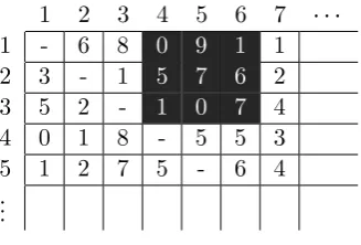
Blocks work differently than counts. If a part of the OD matrix is known, for example from a travel survey, it can be implemented in a block. A block means that the known cells are calibrated together, with the total value of the block. A small example:

1 2 3 4 5 6 7

1 - 6 8 0 9 1 1

2 3 - 1 5 7 6 2

3 5 2 - 1 0 7 4

4 0 1 8 - 5 5 3

5 1 2 7 5 - 6 4

[image:32.595.219.383.156.267.2]

.. .

Figure 3.2: Example of a Block

In the above example all the amount of traffic between centroids 1, 2, 3, and centroids 4, 5, 6 is known, these entries are coloured in grey. The block then also holds the total amount of traffic, and this is taken into account in the calibrations. For the example the block might have a real value of 40, while the cells in the OD matrix only have a value of 36.

• Trip Ends

Trip ends are exactly what the name implies: the ends of a trip (the end can be either the beginning/origin or the end/destination of a trip). If the amount of people arriving at a zone is known, that information can be used to calibrate a whole column of the

OD matrix, °_igij. The same holds for departing people and a row of the OD matrix,

°

jgij:

1 2 3 4 5 6 7

1 - 6 8 0 9 1 1

2 3 - 1 5 7 6 2

3 5 2 - 1 0 7 4

4 0 1 8 - 5 5 3

5 1 2 7 5 - 6 4

.. .

Figure 3.3: Example of a Trip End

3.6.2 Formulas

[image:32.595.217.383.468.576.2]

(33)

Screenline matrices are made for each linkl, and hold information for every OD pair. Each

value of a cell pi, jq lies on the interval r0,1s, and indicate which percentage of the total

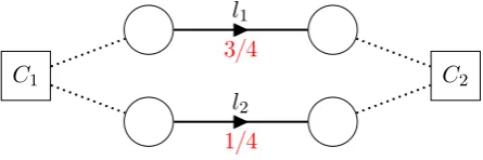
flow going from centroiditoj actually goes across linkl. For example:

C1 C2

I

3{4

l1

I

1{4

[image:33.595.186.409.146.220.2]

l2

Figure 3.4: Example Network

The above example network gives rise to the following screenline matrices:

Sl1

3

4

0

and Sl2

1

4

0

Then OD matrix calibration works by checking every restriction, one after another, and ‘implementing’ them to the starting matrix. A ‘restriction’ is the general term for the data sources mentioned above; counts, screenlines, blocks and trip ends. For each restriction all

OD pairs are calibrated, by multiplying their original value with a calibration factorχ0:

χ0

°

rCr

°

rpgijqr

Here Cr is the value of the rth restriction, and pgijqr the cells in the matrix belonging to

the rth _restriction.

For the actual calibration every restriction is calibrated separately. Each restriction calcu-lates a calibration factor, based on the following formula:

g_ijnewg_ijold

¸ Cr

i,jPr

Pijrgoldij

r

withg_ijnewandgold_ij the new and old values of cellpi, jq,Crthe total value of restrictionr,Pijr

the fraction of the OD pairpi, jq passing restriction r, and r the elasticity of restriction r

(how ‘reliable’ the restriction is).

In the above formula there is no direct mention of v or ˆv. The value of ˆv is of course

the value Cr, and the original value of v is calculated by the sum

°

i,jPrPijrgijold. For this

calculations only the OD flows that are used by the restriction are used: ti, j |vpgi,jq Pru.

In OmniTRANS these four data sources are given different priorities, which can be set by

the user. By default the order of these sources is: BlocksÑ CountsÑ Screenlines ÑTrip

(34)

3.7

Gradient Descend Method

As mentioned in Chapter 2 this thesis also looks at the gradient descend method to solve the problem of calibrating an OD matrix. In particularly the gradient descend method as given by [Smits, 2010] will be used. This version was designed especially for OmniTRANS, and although it is not yet implemented in OmniTRANS, the planning is that this will be done in the near future.

From the literature we have the following general problem description for OD matrix cali-bration:

min

g,l Fpg,lq αF1pg,gq pˆ 1αqF2pl, Cq

s.t. lassignpgq, (GP)

g¥0,

l¥0.

In the above description the formulation of [Smits, 2010] is already used. Herel is the set

of all flows (which used to bev), andC the set of all counted values (which used to be ˆv).

[Smits, 2010] uses for the cost functionsF1 and F2 theL2 norm, after considering several

alternatives. The factor r is reused, to give a weight to each restriction in the objective

function. The above problem is still a bi-level optimization problem (both the assignment

of g and the general problem is an optimization problem). Which means that it is difficult

to solve numerically, and often no good solution is found at all.

To combat this drawback [Smits, 2010] assumes that the assignment of g is locally

pro-portional, meaning that between iterations the route assignment does not change much.

Therefore, with that assumption, the assignment of g doesn’t have to be calculated every

iteration, which makes the problem a single level convex sub-problem of the original:

min

g Fpgq α

¸

pi,jq PI dPD

1 2

gd_ijˆg_ijd 2 p1αq¸ rPR

r

2

¸

pi,jq PI, dPDr

P_ijrd g_ijd Cr

2

s.t. g¥0

In the above formulation D is the set of dimensions (as defined by OmniTRANS,

sec-tion 3.2), Dr is the set of dimensions used by restriction r, I the set of all OD pairs i, j,

and P_ijrd is the fraction of the demand of OD pair pi, jq in dimension d that applies to

restrictionr. The variablesvand ˆv(or land C) are considered implicitly; Cr is the value

(35)

From the gradient descend method [Smits, 2010] devised the following algorithm:

AlgorithmThe OmniTRANS gradient method algorithm 1 : stopCritÐfalse

2 : g Ð˜g

3 : while notstopCrit do

4 : sÐ g∇Fpgq [1]

5 : λð _BB_λFpg λsq 0 [2]

6 : gÐg λs

7 : updatestopCrit

8 : end while

9 : g Ðg [3]

Steps [1] and [2] can be solved algebraically, giving a formula for the solution of s and

λ, respectively. These calculations or the results will not be shown here, for more detail

please consult [Smits, 2010]. In step [1] also the gradient ∇Fpgq is multiplied with the

current OD matrixg. This is done to make sure that OD pairs that are 0 remain so. Some

comments on this approach will be discussed in section 15.2.

One remark must be made concerning [3], given its strange appearance. Because the

al-gorithm itself does not guarantee a positive value for all gij, it has to be forced with an

additional step:

g

!

max

!

0, g_i,jd

)

| pi, jq PI, dPD

)

The above is of course an ugly solution. According to [Smits, 2010]gnever became negative

(36)

4.

Problem Specification

77 77 77 77 77

With the Literature Research done, a lot of different information passed in review. Therefore it is now time to give some more specification of the problem that will be treated in this thesis. In section 4.1 something will be said about the OD matrix calibration in general. Then section 4.2 treats the restrictions that will have to be formulated. And in section 4.3 a look will be taken at routes generated by the data.

4.1

OD Matrix Calibration

As mentioned in section 2.2.2 there are several different solution methods for the problem of OD matrix calibration. At the moment OmniTRANS uses a custom made algorithm, which works by multiplying OD pairs with a factor based on the restrictions added to OmniTRANS (counts, screenlines, blocks and trip ends, as defined in section 3.6). This calibration does not work as good as the people at Omnitrans want, and therefore in the first part of 2010 a large study was made of OD matrix calibrations.

From that study two new algorithms were found, which are described in depth in [Smits, 2010]. The first algorithm is an improved version of the custom algorithm in OmniTRANS, the second is a new algorithm based on a gradient descend method. These two new algo-rithms are not yet implemented in OmniTRANS, but the implementation is planned for the near future. In studying the two algorithms two small errors were found, and these will be changed before the algorithms will be used for this thesis.

The adapted OmniTRANS algorithm uses the same calibration factors as described in section 3.6, but for every OD pair all calibration factors are taken together, by taking the geometric mean of the factors. Because not all factors should be weighted equally, the

geometric mean is weighted withPijr, the percentage of the OD flow passing the restriction.

According to [Smits, 2010] this gives the following formula:

gnew_ij gold_ij

¹

rPR

° Cr

i,jPr gold

ij Pijr

rPijr

1

° rPRr Pijr

But the above formula is not entirely correct. The calibration factors are weighted with the

percentage Pijr, but in the exponent the sum is taken of rPijr, which is incorrect. This

(37)

Therefore the real formula should be:

gnew_ij gold_ij

¹

rPR

° Cr

i,jPr gold

ij Pijr

rPijr

1

° rPRPijr

For the gradient descent method another (small) improvement was found. In [Smits, 2010] the concern was that with the gradient descend method it could happen that cells in the OD matrix became negative. His solution was to truncate all negative cells to 0, at the

end of the calibration. But that means that perhaps not the optimalpositivesolution was

found. Therefore it is better to check the non-negativity in the algorithm itself, leading to the following algorithm:.

AlgorithmThe OmniTRANS gradient method algorithm (2) 1 : stopCritÐfalse

2 : g Ð˜g

3 : while notstopCrit do

4 : sÐ g∇Fpgq

5 : λð _BB_λFpg λsq 0

6 : pλsqij Ðmaxtgij,pλsqiju @i,j

7 : gÐg λs

8 : updatestopCrit

9 : end while

More discussion on this aspect of the gradient method will be treated in Chapter 15.

With the solution method(s) of the OD matrix calibration given, it means that in the rest of this thesis only attention will be given to the data from the public transport and from mobile phones. This data will have to be modelled and converted to a format which can be used for OD matrix calibration.

4.2

Restrictions

The way that information about the real world (traffic counts, surveys, etc.) is used by OD

matrix calibration is with so-called restrictions. Restrictions have a value (Cr) and weight

(r), and a list of OD pairs pi, jq passing that restriction. And because not always the

entire flow of an OD pair passes the restriction, also for every OD pair the fraction of flow

that does pass the restriction is known (Pijr). This also makes it easy to define a general

definition: if an OD pair is not used by the restriction thenPijr0.

For the two algorithms treated above (Improved OmniTRANS and Gradient Descent) the restrictions are taken into account in two different ways. For the adapted OmniTRANS

algorithm the restrictions are taken into account with the calibration factors, _° Cr

i,jgijoldPijr.

For the gradient descent method the restrictions are part of the objective functionF2, by

the distance between v and ˆv. Therefore the restrictions are taken into account when

(38)

At the moment there are four types of restrictions formulated in OmniTRANS: counts, screenlines, blocks and trip ends. These four types are enough when working with informa-tion from traffic counts and surveys. But the expectainforma-tion is that these will not be enough for this thesis. Because the data from the OV-Chipkaart and from mobile phones give more information than traffic counts, more flexible restrictions will be needed. But this is something that will be further discussed in the modelling chapters of the OV-Chipkaart data (Chapter 5) and the mobile phone data (Chapter 10).

4.3

Routes

Something that has not been mentioned before, but is of some importance, is that the data of mobile phones can perhaps generate more data than just an OD matrix calibration. A dataset from a mobile phone provider shows the actual route that the mobile phone took, not just an origin and destination. Therefore it would be a waste not to use that information. Using the routes from mobile phone datasets is of course no longer part of OD matrix calibration, and therefore it will be studied how routes can be best inserted into the research of this thesis.

(39)

Part I

(40)

5.

Modelling OV-Chipkaart data

77 77 77 77 77 77

Now that the background of the project has been treated it is time for the modelling phase. In this chapter a start will be made with modelling the OV-Chipkaart data. In section 5.1 first something will be said about how public transport data is used in the literature. Then in section 5.2 a look will be taken into the structure of the data from the OV-Chipkaart. And in section 5.3 the first step will be taken in the modelling, resulting in three different approaches.

5.1

Other Literature

In the Literature Review (Chapter 2) several publications were found dealing with the problem of OD matrix calibration. Most of these publications however made no reference to using data from public transport. In the calibration of OD matrices mainly traffic counts are used, and traffic counts are only available for cars, not for public transport passengers. Of course some publications have such a general problem description, that public transport could easily be included. This general description however doesn’t give any insight as to how public transport data should be structured or used. Therefore not much is known about using public transport data for the calibration of OD matrices.

Two papers that do explicitly use public transport data for OD matrix calibration are: [Cui, 2006] and [Chan, 2007]. In these papers the OD matrices were calibrated with infor-mation from the London Underground and the Chicago bus network, respectively. The big

difference between those papers and the situation used in this thesis is that they use only

data from the public transport, they model the transit lines as a closed circuit without any influence from other modes. This has as effect that the stops (stations) are modelled as the zones, and therefore all data from one stop to another is taken into account, as it is exactly the traffic between one OD pair.

(41)

Without any pre-existing research to build on, the whole modelling phase will begin with an examination of the data structure, as it is provided by the OV-Chipkaart.

5.2

Data Structure

The data generated by the OV-Chipkaart is the collection of all journeys made by people in the public transport. Every time a person checks in at the start of his or her journey the starting stop is stored, and when the person checks out again the final stop is added, creating a whole journey. The collection of all these journeys is of course aggregated, for a certain time period, to remove any personal information.

There are three types of journeys that are stored by the OV-Chipkaart:

• A complete journey

• Zero travel distance

• Only a check-in

From these three only the complete journey is of use. The zero travel distance implies that a person entered a station and left again, without actually travelling through the network. Zero travel distances happens for example when people come to collect someone. As no actual journey is made, these results are ignored.

With only a check-in the destination of a journey is unknown. Only a check-in happens if a person forgets to check-out at the final stop, or checks out without having checked in (in that case the system considers it a check-in). If the destination of a trip is missing not much can be said about that trip. There have been publishings trying to find the whole trip, but the results vary per situation. And as the assumption is that this will not happen very often, these types are also ignored.

The results from the complete journeys are aggregated, and give rise to a large matrixH,

showing the number of journeys from one stop to another in a certain time period (for

example one hour). To illustrate: the cell Hpf, kq contains the number of people checking

in at stopf, and checking out at stopk. The cells Hpf, fq are all empty, as zero distance

journeys are ignored. Because the results in the matrix H are aggregated already some

information is lost. For example a transfer to another transit line counts as two separate journeys, and therefore the information about the entire journey is lost, and only the separate parts are known.

(42)

There is one important aspect that influences the quality of OV-Chipkaart data, namely the fact if the OV-Chipkaart is the only valid payment option, or if there are still other methods. If the OV-Chipkaart is the only valid payment option the data is complete, it shows all journeys made with the public transport. But in the case that there are still other valid payment options, the data becomes incomplete, as not all journeys are tracked. In that case another approach must be used, to be able to use the data.

5.3

Initial Modelling

With the structure of the OV-Chipkaart data defined, a begin can be made with the model-ling of OV-Chipkaart data.

5.3.1 Converting to Counts

In OmniTRANS all traffic data that is used for OD calibration is entered as a count on a link. Therefore the first step in the OV-Chipkaart modelling is to see if the definition of

counts can also be used for OV-Chipkaart data. The information in matrixH is of course

based on stops, not on links. When all transit lines and their stops are known (and it is

assumed that this is the case), the numbers from the matrix H can be added to create a

count for every link between two stops. For the calculation of counts an easy algorithm can be written (see section 6.2) with which this could be done.

If all data from the matrix H is converted to counts, it means that a lot of information is

lost. With counts it is only known that a certain number of people passed that link, but

the data from the matrix H also says something about where passengers came from and

where they went after. It also means that that particular count is used to calibrate all OD pairs that have a path crossing it. While perhaps if the full journey was known, only one OD pair would fit that journey, and therefore the other OD pairs were wrongly calibrated.

These objections mean that OV-Chipkaart data cannotjust be converted to counts,

some-thing else has to be done to preserve the extra information from the matrixH.

5.3.2 Routes

The second approach to modelling the OV-Chipkaart dat