When and why are log linear models self normalizing?

When and why are log-linear models self-normalizing?

Computer Science Division University of California, Berkeley {jda,klein}@cs.berkeley.edu

Abstract

Several techniques have recently been pro-posed for training “self-normalized” discrimi-native models. These attempt to find parameter settings for which unnormalized model scores approximate the true label probability. How-ever, the theoretical properties of such tech-niques (and of self-normalization generally) have not been investigated. This paper exam-ines the conditions under which we can ex-pect self-normalization to work. We character-ize a general class of distributions that admit self-normalization, and prove generalization bounds for procedures that minimize empiri-cal normalizer variance. Motivated by these results, we describe a novel variant of an estab-lished procedure for training self-normalized models. The new procedure avoids computing normalizers for most training examples, and decreases training time by as much as factor of ten while preserving model quality.

1 Introduction

This paper investigates the theoretical properties of log-linear models trained to make their unnormalized scores approximately sum to one.

Recent years have seen a resurgence of interest in log-linear approaches to language modeling. This includes both conventional log-linear models (Rosen-feld, 1994; Biadsy et al., 2014) and neural networks with a log-linear output layer (Bengio et al., 2006). On a variety of tasks, these LMs have produced sub-stantial gains over conventional generative models based on countingn-grams. Successes include ma-chine translation (Devlin et al., 2014) and speech recognition (Graves et al., 2013). However, log-linear LMs come at a significant cost for computational ef-ficiency. In order to output a well-formed probability distribution over words, such models must typically calculate a normalizing constant whose computa-tional cost grows linearly in the size of the vocab-ulary.

Fortunately, many applications of LMs remain well-behaved even if LM scores do not actually cor-respond to probability distributions. For example, if a machine translation decoder uses output from a pre-trained LM as a feature inside a larger model, it suffices to have all output scores on approximately the same scale, even if these do not sum to one for every LM context. There has thus been considerable research interest around training procedures capa-ble of ensuring that unnormalized outputs for every context are “close” to a probability distribution. We are aware of at least two such techniques: noise-contrastive estimation (NCE) (Vaswani et al., 2013; Gutmann and Hyv¨arinen, 2010) and explicit penal-ization of the log-normalizer (Devlin et al., 2014). Both approaches have advantages and disadvantages. NCE allows fast training by dispensing with the need to ever compute a normalizer. Explicit penalization requires full normalizers to be computed during train-ing but parameterizes the relative importance of the likelihood and the “sum-to-one” constraint, allowing system designers to tune the objective for optimal performance.

While both NCE and explicit penalization are ob-served to work in practice, their theoretical properties have not been investigated. It is a classical result that empirical minimization ofclassification erroryields models whose predictions generalize well. This pa-per instead investigates a notion ofnormalization error, and attempts to understand the conditions un-der which unnormalized model scores are a reliable surrogate for probabilities. While language model-ing serves as a motivation and runnmodel-ing example, our results apply to any log-linear model, and may be of general use for efficient classification and decoding. Our goals are twofold: primarily, to provide intu-ition about how self-normalization works, and why it behaves as observed; secondarily, to back these intu-itions with formal guarantees, both about classes of normalizable distributions and parameter estimation procedures. The paper is built around two questions:

Whencan self-normalization work—for which dis-tributions do good parameter settings exist? And whyshould self-normalization work—how does ance of the normalizer on held-out data relate to vari-ance of the normalizer during training? Analysis of these questions suggests an improvement to the training procedure described by Devlin et al., and we conclude with empirical results demonstrating that our new procedure can reduce training time for self-normalized models by an order of magnitude. 2 Preliminaries

Consider a log-linear model of the form

p(y|x;θ) = Pexp{θy>x}

y0exp{θ>_y0x} (1)

We can think of this as a function from acontextxto a probability distribution overdecisionsyi, where each

decision is parameterized by a weight vectorθy.1For

concreteness, consider a language modeling problem in which we are trying to predict the next word after the context the ostrich. Herex is a vector of fea-tures on the context (e.g.x={1-2=the ostrich, 1=the, 2=ostrich,. . .}), andyranges over the full vocabulary (e.g.y1 =the,y2 =runs, . . . ).

Our analysis will focus on the standard log-linear case, though later in the paper we will also relate these results to neural networks. We are specifically concerned with the behavior of the normalizer or partition function

Z(x;θ)def₌X

y

exp{θ>_yx} (2)

and in particular with choices of θ for which Z(x;θ)≈1for mostx.

To formalize the questions in the title of this paper, we introduce the following definitions:

Definition 1. A log-linear modelp(y|x,θ) is

nor-malizedwith respect to a setX if for everyx ∈ X, Z(x;θ) = 1. In this case we callX normalizable andθnormalizing.

Now we can state our questions precisely: What distributions are normalizable? Given data points 1_{An alternative, equivalent formulation has a single weight} vector and a feature function from contexts and decisions onto feature vectors.

Figure 1: A normalizable set, the solutions [x, y] to

Z([x, y];{[−1,1],[−1,−2]}) = 1. The set forms a smooth one-dimensional manifold bounded on either side by the hyperplanes normal to[−1,1]and[−1,−2].

from a normalizableX, how do we find a normalizing

θ?

In sections 3 and 4, we do not analyze whether the setting ofθcorresponds to a good classifier—only a good normalizer. In practice we require both good normalizationandgood classification; in section 5 we provide empirical evidence that both are achiev-able.

Some notation: Weight vectorsθ(and feature vec-torsx) ared-dimensional. There arekoutput classes, so the total number of parameters inθiskd. || · ||p

is the`pvector norm, and|| · ||∞specifically is the max norm.

3 When should self-normalization work? In this section, we characterize a large class of datasets (i.e. distributions p(y|x)) that are normal-izable either exactly, or approximately in terms of their marginal distribution overcontextsp(x). We begin by noting simple features of Equation 2: it is convex inx, so in particular its level sets enclose con-vex regions, and are manifolds of lower dimension than the embedding space.

As our definition of normalizability requires the existence of a normalizingθ, it makes sense to begin by fixingθand considering contextsxfor which it is normalizing.

Observation. Solutions x to Z(x;θ) = 1, if any

This follows immediately from the definition of a convex function, but provides a concrete example of a set for whichθis normalizing: the solution set of Z(x;θ) = 1has a simple geometric interpretation as a particular kind of smooth surface. An example is depicted in Figure 1.

We cannot expect real datasets to be this well be-haved, so seems reasonable to ask whether “good-enough” self-normalization is possible for datasets (i.e. distributionsp(x)) which are only close to some exactly normalizable distribution.

Definition 2. A context distributionp(x)isD-close

to a setX if

Ep

inf

x∗_∈X||X−x ∗_||

∞

=D (3)

Definition 3. A context distribution p(x) is ε

-approximately normalizableifEp|logZ(X;θ)| ≤ε.

Theorem 1. Suppose p(x) is D-close to {x :

Z(x;θ) = 1}, and each ||θi||∞ ≤ B. Then p(x) isdBD-approximately normalizable.

Proof sketch.2 _{Represent each X as X}∗ _{+ X}−_, whereX∗_{solves the optimization problem in} Equa-tion 3. Then it is possible to bound the normalizer by log exp{θ˜>_X−_{}, whereθ}˜_{maximizes the magnitude} of the inner product withX−_overθ.

In keeping with intuition, data distributions that are close to normalizable sets are themselves approx-imately normalizable on the same scale.3

4 Why should self-normalization work? So far we have given a picture of what approxi-mately normalizable distributions look like, but noth-ing about how to find normaliznoth-ingθ from training data in practice. In this section we prove that any pro-cedure that causes training contexts to approximately normalize will also have log-normalizers close to zero in unseen contexts. As noted in the introduction, this does not follow immediately from correspond-ing results forclassificationwith log-linear models. While the two problems are related (it would be quite surprising to have uniform convergence for classifi-cation but not normalization), we nonetheless have a

2_{Full proofs of all results may be found in the Appendix.} 3_{Here (and throughout) it is straightforward to replace} quan-tities of the formdBwithBby working in`2instead of`∞.

different function class and a different loss, and need new analysis.

Theorem 2. Consider a sample(X1, X2, . . .), with

all||X||∞ ≤R, andθwith each||θi||∞≤ B. Ad-ditionally define Lˆ = 1

n

P

i|logZ(Xi)|and L =

E|logZ(X)|. Then with probability1−δ,

|L − L| ≤ˆ 2

s

dk(logdBR+ logn) + log1

δ

2n +

2

n (4)

Proof sketch. Empirical process theory provides standard bounds of the form of Equation 4 (Kakade, 2011) in terms of the size of acoverof the function class under consideration (hereZ(·;θ)). In particu-lar, given someα, we must construct a finite set of

ˆ

Z(·;θ) such that someZˆ is everywhere a distance of at mostα from everyZ. To provide this cover, it suffices to provide a cover ˆθ forθ. If the ˆθ are spaced at intervals of lengthD, the size of the cover is(B/D)kd_{, from which the given bound follows.}

This result applies uniformly across choices ofθ

regardless of the training procedure used—in partic-ular,θcan be found with NCE, explicit penalization, or the variant described in the next section.

As hoped, sample complexity grows as the number of features, and not the number of contexts. In partic-ular, skip-gram models that treat context words inde-pendently will have sample efficiency multiplicative, rather than exponential, in the size of the condition-ing context. Moreover, if some features are correlated (so that data points lie in a subspace smaller thand dimensions), similar techniques can be used to prove that sample requirements depend only on this effec-tive dimension, and not the true feature vector size.

We emphasize again that this result says nothing about thequalityof the self-normalized model (e.g. the likelihood it assigns to held-out data). We de-fer a theoretical treatment of that question to future work. In the following section, however, we provide experimental evidence that self-normalization does not significantly degrade model quality.

5 Applications

normalizer for each training example, or at least keep-ing track of an estimate of the normalizer for each training example.

Our results here suggest that it should be possi-ble to obtain approximate self-normalizing behavior withoutanyrepresentation of the normalizer on some training examples—as long as a sufficiently large fraction of training examples are normalized, then we have some guarantee that with high probability the normalizer will be close to one on the remaining training examples as well. Thus an unnormalized likelihood objective, coupled with a penalty term that looks at only a small number of normalizers, might nonetheless produce a good model. This suggests the following:

l(θ) =X

i

θ>_yixi+ α_γ

X

h∈H

(logZ(xh;θ))2 (5)

where the parameter α controls the relative impor-tance of the self-normalizing constraint, H is the set of indices to which the constraint should be ap-plied, andγcontrols the size ofH, with|H|=dnγe. Unlike the objective used by Devlin et al. (2014) most examples arenevernormalized during training. Our approach combines the best properties of the two techniques for self-normalization previously dis-cussed: like NCE, it does not require computation of the normalizer on all training examples, but like ex-plicit penalization it allows fine-grained control over the tradeoff between the likelihood and the quality of the approximation to the normalizer.

We evaluate the usefulness of this objective with a set of small language modeling experiments. We train a log-linear LM with features similar to Biadsy et al. (2014) on a small prefix of the Europarl cor-pus of approximately 10M words.4 _{We optimize the}

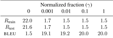
objective in Equation 5 using Adagrad (Duchi et al., 2011). The normalized setHis chosen randomly for each new minibatch. We evaluate using two metrics: BLEUon a downstream machine translation task, and normalization riskR, the average magnitude of the log-normalizer on held-out data. We measure the re-sponse of our training to changes inγandα. Results are shown in Table 1 and Table 2.

4_{This prefix was chosen to give the fully-normalized model} time to finish training, allowing a complete comparison. Due to the limited LM training data, these translation results are far from state-of-the-art.

Normalized fraction (γ)

0 0.001 0.01 0.1 1

Rtrain 22.0 1.7 1.5 1.5 1.5

Rtest 21.6 1.7 1.5 1.5 1.5

BLEU 1.5 19.1 19.2 20.0 20.0

Table 1: Result of varying normalized fractionγ, with

α= 1. When no normalization is applied, the model’s be-havior is pathological, but when normalizing only a small fraction of the training set, performance on the down-stream translation task remains good.

Normalization strength (α)

α 0.01 0.1 1 10

Rtrain 20.4 9.7 1.5 0.5

Rtest 20.1 9.7 1.5 0.5

BLEU 1.5 2.6 20.0 16.9

Table 2: Result of varying normalization parameterα, withγ= 0.1. Normalization either too weak or too strong results in poor performance on the translation task, em-phasizing the importance of training procedures with a tunable normalization parameter.

Table 1 shows that with small enoughα, normal-ization risk grows quite large. Table 2 shows that forcing the risk closer to zero is not necessarily desir-able for a downstream machine translation task. As can be seen, no noticeable performance penalty is incurred when normalizing only a tenth of the train-ing set. Performance gains are considerable: setttrain-ing γ = 0.1, we observe a roughly tenfold speedup over γ = 1.

On this corpus, the original training procedure of Devlin et al. withα = 0.1 gives a BLEU score of 20.1 and Rtest of 2.7. Training time is equivalent

to choosing γ = 1, and larger values of α result in decreasedBLEU, while smaller values result in significantly increased normalizer risk. Thus we see that we can achieve smaller normalizer variance and an order-of-magnitude decrease in training time with a loss of only0.1BLEU.

6 Relation to neural networks

comes from deeper networks. All of the proof tech-niques used in this paper can be combined straight-forwardly with existing tools for covering the out-put spaces of neural networks (Anthony and Bartlett, 2009). If optimization of the self-normalizing portion of the objective is deferred to a post-processing step after standard (likelihood) training, and restricted to parameters in the output layers, then Theorem 2 applies exactly.

7 Conclusion

We have provided both qualitative and formal charac-terizations of “self-normalizing” log-linear models, including what we believe to be the first theoretical guarantees for self-normalizing training procedures. Motivated by these results, we have described a novel objective for training self-normalized log-linear mod-els, and demonstrated that this objective achieves significant performance improvements without a de-crease in the quality of the models learned.

A Quality of the approximation

Proof of Theorem 1. Using the definitions of X∗_, X−_andθ˜_{given in the proof sketch for Theorem 1,}

E|log(Xexp{θ>

i X})|

=E|log(Xexp{θ>

i (X∗+X−)})|

≤E|log(exp{θ˜>X−}Xexp{θ>_i X∗})| ≤E|log(exp{θ˜>X−})|

≤dDB

B Generalization error

Lemma 3. For anyθ1, θ2 with||θ1,i−θ2,i||∞ ≤

Ddef_{=α/dRfor alli,}

||logZ(x;θ1)| − |logZ(x;θ2)|| ≤α (6)

Proof.

||logZ(x;θ1)| − |logZ(x;θ2)||

≤ |logZ(x;θ1)−logZ(x;θ2)|

≤logZ(x;θ1)

Z(x;θ2) (w.l.o.g.)

= log

P

iexp

(θ_P1i−θ2i)>x expθ>2ix iexp

θ> 2ix

≤dDR+ logZ_Z(₍x_x;_;θ_θ2) 2) =α

Corollary 4. The set of partition functions Z =

{Z(·;θ) : ||θ||∞ ≤ B ∀θ ∈ θ} can be covered on on the`∞ ball of radiusR by a grid ofθˆ with distanceD. The size of this cover is

|Z|ˆ =

B D

_dk

=

dBR α

_dk

(7)

Proof of Theorem 2. From a standard discretization lemma (Kakade, 2011) and Corollary 4, we immedi-ately have that with probabilty1−δ,

sup

Z∈Z| ˆ

L − L| ≤

≤inf

α 2

s

dk(logdBR−logα) + log1

δ

2n + 2α

Takingα = 1/n,

≤2

s

dk(logdBR+ logn) + log1

δ

2n +

2 n Acknowledgements

The authors would like to thank Peter Bartlett, Robert Nishihara and Maxim Rabinovich for useful discus-sions. This work was partially supported by BBN under DARPA contract HR0011-12-C-0014. The first author is supported by a National Science Foun-dation Graduate Fellowship.

References

Martin Anthony and Peter Bartlett. 2009. Neural net-work learning: theoretical foundations. Cambridge University Press.

Fadi Biadsy, Keith Hall, Pedro Moreno, and Brian Roark. 2014. Backoff inspired features for maximum entropy language models. InProceedings of the Conference of the International Speech Communication Association. Jacob Devlin, Rabih Zbib, Zhongqiang Huang, Thomas Lamar, Richard Schwartz, and John Makhoul. 2014. Fast and robust neural network joint models for statisti-cal machine translation. InProceedings of the Annual Meeting of the Association for Computational Linguis-tics.

John Duchi, Elad Hazan, and Yoram Singer. 2011. Adaptive subgradient methods for online learning and stochastic optimization. Journal of Machine Learning Research, 12:2121–2159.

Alex Graves, Navdeep Jaitly, and Abdel-rahman Mo-hamed. 2013. Hybrid speech recognition with deep bidirectional LSTM. InIEEE Workshop on Automatic Speech Recognition and Understanding, pages 273– 278.

Michael Gutmann and Aapo Hyv¨arinen. 2010. Noise-contrastive estimation: A new estimation principle for unnormalized statistical models. InProceedings of the International Conference on Artificial Intelligence and Statistics, pages 297–304.

Sham Kakade. 2011. Uniform and empirical cov-ering numbers. http://stat.wharton. upenn.edu/˜skakade/courses/stat928/ lectures/lecture16.pdf.

Ronald Rosenfeld. 1994. Adaptive statistical language modeling: a maximum entropy approach. Ph.D. thesis. Ashish Vaswani, Yinggong Zhao, Victoria Fossum, and