Lexicon Integrated CNN Models with Attention for Sentiment Analysis

Lexicon Integrated CNN Models with Attention for Sentiment Analysis

Bonggun Shin, Timothy Lee, Jinho D. Choi Math and Computer Science

Emory University Atlanta, GA 30322

{bonggun.shin,timothy.lee,jinho.choi}@emory.edu

Abstract

With the advent of word embeddings, lex-icons are no longer fully utilized for sen-timent analysis although they still provide important features in the traditional setting. This paper introduces a novel approach to sentiment analysis that integrates lexicon embeddings and an attention mechanism into Convolutional Neural Networks. Our approach performs separate convolutions for word and lexicon embeddings and pro-vides a global view of the document using attention. Our models are experimented on both the SemEval’16 Task 4 dataset and the Stanford Sentiment Treebank and show comparative or better results against the existing state-of-the-art systems. Our analysis shows that lexicon embeddings al-low building high-performing models with much smaller word embeddings, and the attention mechanism effectively dims out noisy words for sentiment analysis.

1 Introduction

Sentiment analysis is a task of identifying senti-ment polarities expressed in docusenti-ments, typically positive, neutral, or negative. Although the task of sentiment analysis has been well-explored (Mullen and Collier, 2004; Pang and Lee, 2005; Wilson et al.,2005), it is still very challenging due to the complexity of extracting human emotion from raw text. The recent advance of deep learning has defi-nitely elevated the performance of this task (Socher et al.,2013;Kim,2014;Yin and Sch¨utze, 2015) although there is much more room to improve.

In the traditional setting where statistical models are based on sparse features, lexicons consisting of words and their sentiment scores are shown to be highly effective for sentiment analysis because

they provide features that may not be captured from training data (Hu and Liu,2004;Kim and Hovy,

2004;Ding et al.,2008;Taboada et al.,2011). How-ever, since the appearance of word embeddings, the use of lexicons is getting faded away because word embeddings are believed to capture the sentiment aspects of those words. This brought us two impor-tant questions:

• Can lexicons be still useful for sentiment anal-ysis when coupled with word embeddings? • If yes, what is the most effective way of

incor-porating lexicons with word embeddings? To answer these questions, we first construct lexi-con embeddings that are specifically designed for sentiment analysis and integrate them into the exist-ing Convolutional Neural Network (CNN) model similar toKim(2014). Three ways of lexicon in-tegration to the CNN model are proposed, which show distinctive characteristics for different gen-res (Section3.2). We then incorporate an efficient attention mechanism to our CNN models, which provides a global view of the document by em-phasizing (or de-emem-phasizing) important words and lexicons (Section3.3). Our models using lexi-con embeddings are evaluated on two well-known datasets, the SemEval’16 dataset and the Stanford Sentiment Treebank, and show state-of-the-art re-sults on both datasets (Section4). To the best of our knowledge, this is the first time that lexicon embeddings are introduced for sentiment analysis.

2 Related Work

The first attempt of sentiment analysis on text was initiated byPang et al.(2002) who pioneered this field by using bag-of-word features. This work mostly hinged on feature engineering; since then, many kinds of feature learning methods had been introduced to increase the performance (Pang and

Lee,2008;Liu,2012;Gimpel et al., 2011; Feld-man,2013;Mohammad et al.,2013b). Aside from pure machine learning approaches, lexicon based approaches had been another trend, which relied on the manual or algorithmic creation of word sen-timent scores (Hu and Liu,2004;Kim and Hovy,

2004;Ding et al.,2008;Taboada et al.,2011). Since the emergence of the Convolutional Neu-ral Networks (CNN;Collobert et al.(2011)), con-ventional methods have become gradually obso-lete because of the outstanding performance from the CNN variants. CNN based models are distin-guished from earlier methods because they do not rely on laborious feature engineering. The first success of CNN in sentiment analysis was trig-gered by document classification research (Kim,

2014), where CNN showed state-of-the-art results in numerous document classification datasets. This success has engendered an upsurge in deep neural network research for sentiment analysis. Various modified models have been proposed in the litera-ture. One of the famous deep learning methods that models a document is the generalized phrase pro-posed byYin and Sch¨utze(2014), which represents a sentence using element-wise addition, multiplica-tion, or recursive auto-encoder.

Endeavors to capturen-gram information bore fruits with CNN, max pooling, and softmax ( Col-lobert et al.,2011;Kim,2014), which is regarded as the standard methods of the document classification problem these days. Kalchbrenner et al. (2014a) extended this standard CNN model with dynamic k-max pooling, which served as an input layer to another stacked convolution layer. Multichannel CNN methods (Kim,2014;Yin and Sch¨utze,2015) are another branch of CNN, where assorted embed-dings are considered together when convolving the input. UnlikeKim(2014)’s model that relies on a single type of embedding with different mutability characteristics of the weights of embedding layer,

Yin and Sch¨utze(2015) incorporates diverse sort of embedding types using multichannel CNN.

Two notable pioneers in using lexicon for senti-ment analysis areMohammad et al.(2013a); Kalch-brenner et al.(2014b) generated scores with other manually generated sentiment lexicon scores to achieved the state-of-the-art result in SemEval-2013 Twitter sentiment analysis task. In general domain,Hu and Liu(2004) generated a user review lexicon that showed promising result in capturing sentiment in customer product reviews.

Attention based methods have been successful in many application domains, such as image classifi-cation (Stollenga et al.,2014), image caption gen-eration (Xu et al.,2015), machine translation (Cho et al., 2014;Bahdanau et al.,2014;Luong et al.,

2015), and question answering (Shih et al.,2016;

Chen et al., 2015; Yang et al., 2016). However, in the field of sentiment analysis, the attention is applied to only aspect-based sentiment classifica-tion (Yanase et al.,2016). To the best knowledge of ours, there is no attention-based model for a general sentiment analysis task.

3 Approach

The models proposed here are based on a convo-lutional architecture and use naive concatenation (Section3.2.1), multichannel (Section3.2.2), sep-arate convolution (Section3.2.3), and embedding attention (Section3.3) for the integration of lexicon embeddings to CNN.

3.1 Baseline

Our baseline approach is a one-layer CNN model using pre-trained word embeddings, which is a reimplementation of the CNN model introduced by

Kim(2014). Lets∈Rn×d_{be a matrix}

represent-ing the input document, wherenis the number of words,dis the dimension of the word embeddings, and each row corresponds to the word embedding, wi ∈ Rd, wherewiindicates thei’th word in the

document. This document matrixsis fed into the convolutional layer and convolved by the weights c∈Rl×d_{, wherelis the length of the filter.}

The convolutional layer can takem-number of filters of the lengthl. Each convolution produces a vectorvc∈Rn−l+1, where elements invcconvey

thel-gram features across the document. The max pooling layer selects the most salient features from each of themvectors produced by the filters. As a result, the output of this max pooling layer is a vec-torvm ∈ R(n−l+1)×m. The selected features are

passed onto the softmax layer, which is optimized for the score of each sentiment class label.

3.2 Lexicon Integration

scores range between−1and1, where−1and1

being the most negative and positive, respectively. However, some lexicons contain non-probabilistic scores (e.g., frequency counts of the word in senti-mental contexts), which are normalized to[−1,1].

(a) Naive concatenation (Section3.2.1). The lexicon embeddings (on the right) are concatenated to the word embeddings (on the left).

(b) Multichannel (Section3.2.2). The lexicon embed-dings are added to the second channel whereas the word embeddings are added to the first channel.

(c) Separate convolution (Section3.2.3). The lexicon embeddings are processed by a separate convolution (on the right) from the word embeddings (on the left). Figure 1: Lexicon integration to the CNN model.

For each wordw∈ W, whereW is the union of all words in the lexicon datasets, a lexicon embed-ding is constructed by concatenating all the scores among the datasets with respect tow. If wdoes not appear in certain datasets,0values are assigned in place. The resulting embedding is in the form of a vectorv∈Re_{, whereeis the total number of}

scores across all lexicon datasets. The following subsections propose three methods for lexicon inte-gration to the baseline CNN model (Section3.1), which depict different characteristics depending on the peculiarities of each domain.

3.2.1 Naive Concatenation

The simplest way of blending a lexicon embedding into its corresponding word embedding is to append

it to the end of the word embedding (Figure1(a)). In a formal notation, the document matrix becomes s∈Rn×(d+e)_{. The subsequent process is the same} as the baseline approach.

3.2.2 Multichannel

Inspired byYin and Sch¨utze(2015) who integrated several kinds of word embeddings using multichan-nel CNN, lexicon embeddings in this approach are represented in another channel along with the word embedding channel where both channels are con-volved together (Figure1(b)). Since the dimension of lexicon embeddings is considerably smaller than that of word embeddings (i.e.,d e), zeros are padded to the lexicon embeddings so their dimen-sions match (i.e.,d= e). The identical shape of these two channels allows multichannel convolu-tion to the input document.

3.2.3 Separate Convolution

Another way of adding lexicon embeddings to the CNN model is to process a separate convolution for them (Figure1(c)). In this case, two individual con-volutions are applied to word embeddings and lexi-con embeddings. The max pooled output features from each convolution are then merged together to form an input vector to the softmax layer. Formally, letlw,lxbe the filter lengths for word embeddings

and lexicon embeddings, respectively. Letmwand

mxbe the numbers of filters for word embeddings

and lexicon embeddings, respectively. The result-ing penultimate layer includes max pooled features from word embeddings and lexicon embeddings of size[(n−lw+ 1)×mw] + [(n−lx+ 1)×mx].

3.3 Embedding Attention

Section3.2describes how lexicon embeddings can be incorporated into the CNN model in Section3.1. Each CNN model uses several filters with different lengths; given the filter lengthl, the convolution considersl-gram features. However, thesel-gram features account only for local views, not the global view of the document, which is necessary for sev-eral transitional cases such as negation in sentiment analysis (Socher et al.,2012). To ameliorate this issue, we introduce the embedding attention vector (EAV), which transforms the document matrix in each embedding space into a vector. For example, the EAV in the word embedding space is calculated as a weighted sum of each column in the document matrixs ∈ Rn×d_{, which yields a vectorv ∈ R}d_.

from the document matrix consisting of word em-beddings and the other from the one consisting of lexicon embeddings. All embeddings in the doc-ument matrix are used to create the EAV through multiple convolutions and max pooling as follows:

1. Applym-number of convolutions with the fil-ter length1to the document matrixs∈Rn×d_.

For lexicon embeddings, the document matrix has a dimension ofRn×e_.

2. Aggregate all convolution outputs to form an attention matrixsa ∈Rn×m, wherenis the

number of words in the document, andmis the number of filters whose length is1. 3. Execute max pooling for each row of the

atten-tion matrixsa, which generates the attention

vectorva∈Rn(Figure2(a)).

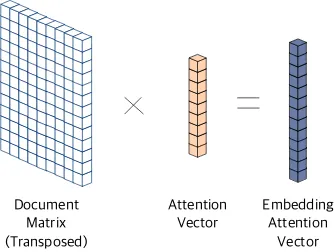
4. Transpose the document matrix ssuch that sT _∈Rd×n_{, and multiply it with the attention}

vectorva∈Rn, which generates the

embed-ding attention vectorve∈Rd(Figure2(b)).

Document

Matrix Attention Matrix(Filter Lenth=1)

Attention Vector (MaxPool)

(a) Given a document matrix, the attention matrix is first created by performing multiple convolutions. The atten-tion vector is then created by performing max pooling on each row of the attention matrix.

Document Matrix (Transposed)

Attention

Vector EmbeddingAttention Vector

(b) The embedding attention vector is created by multiplying the transposed document matrix to the attention vector.

Figure 2: Construction of the embedding attention vector from a document matrix.

The resulting EAVs are appended to the penulti-mate layer to serve as additional information for the softmax layer. For our experiments, EAVs are

generated from both word and lexicon embedding spaces for all of the three lexicon integration meth-ods in Section3.2.

4 Experiments 4.1 Corpora

4.1.1 SemEval-2016 Task 4

All models are evaluated on the micro-blog dataset distributed by the SemEval’16 Task 4a (Nakov et al.,2016). The dataset is gleaned from tweets with annotation of three sentiment classes: posi-tive, neutral, and negative. The available dataset contains only tweet IDs and their sentiment polari-ties; the actual tweet texts are not included in this dataset due to the copyright restrictions. Although the download script provided by SemEval’16 gives a way of accessing the actual texts on the web, a portion of tweets is no longer accessible. To com-pensate this loss, the dataset also includes tweet instances from the SemEval’13 task.

+ 0 - All

TRN 6,480 6,577 2,328 15,385

DEV 786 548 254 1,588

TST 7,059 10,342 3,231 20,632 Table 1: Statistics of the SemEval’16 Task 4 dataset.

+/0/-: positive/neutral/negative, TRN/DEV/TST: training, development, evaluation sets.

The classification results are evaluated by averag-ing the F1-scores of positive and negative senti-ments as suggested by the SemEval’16 Task 4a.

4.1.2 Stanford Sentiment Treebank

Another dataset consisting of movie reviews from Rotten Tomatoes is used for evaluating the robust-ness of our models across different genres. This dataset, called the Stanford Sentiment Treebank, was originally collected byPang and Lee(2005) and later extended bySocher et al.(2013). The sentiment annotation in this dataset is categorized into five classes: very positive, positive, neutral, negative, and very negative. Following the previ-ous work (Kim,2014), the results are evaluated by the conventional classification accuracy.

++ + 0 - – All

TRN 1288 2322 1624 2218 1092 8,544

DEV 165 279 229 289 139 1,101

TST 399 510 389 633 279 2,210

4.2 Embedding Construction 4.2.1 Word Embeddings

To best capture the word semantics in each genre, different corpora are used to train word embed-dings for the SemEval’16 (S16) and the Stanford Sentiment Treebank (SST) datasets. For S16, word embeddings are trained on tweets collected by the Archive Team,1 _{consisting of 3.67M word types.} For SST, word embeddings are trained on the Ama-zon Review dataset,2_{containing 2.67M word types.} All documents are pre-tokenized by the open-source toolkit, NLP4J.3_{The word embeddings are} trained by the original implementation of word2vec from Google using skip-gram and negative sam-pling.4 _{No explicit hyparameter tuning is} per-formed. For each genre, four sets of embeddings with different dimensions (50, 100, 200, 400) are trained to observe the impact of the embedding size on each approach.

4.2.2 Lexicon Embeddings

Six types of sentiment lexicons are used to build lexicon embeddings. All lexicons include senti-ment scores; some lexicons contain information about the frequency of positive and negative senti-ment polarity associated with each word:

• National Research Council Canada (NRC) Hashtag Affirmative and Negated Context Sentiment Lexicon (Kiritchenko et al.,2014). • NRC Hashtag Sentiment Lexicon

(Mohammad et al.,2013a). • NRC Sentiment140 Lexicon

(Kiritchenko et al.,2014). • Sentiment140 Lexicon

(Mohammad et al.,2013a).

• MaxDiff Twitter Sentiment Lexicon (Kiritchenko et al.,2014).

• Bing Liu Opinion Lexicon (Hu and Liu,2004).

When creating lexicon embeddings, the narrow cov-erage of vocabulary in lexicons often raises missing scores. If a given word is missing in a specific lexi-con, neutral scores of 0 are substituted.

1_{archive.org/details/twitterstream} 2_{snap.stanford.edu/data/web-Amazon.html} 3_{github.com/emorynlp/nlp4j}

4_{code.google.com/p/word2vec}

Table3shows the word type coverage of our word and lexicon embeddings for each dataset. The lex-icon embeddings show relatively poor coverage; nevertheless, our experiments show that these lex-icon embeddings help sentiment classification in various ways (Section4.3).

Word Emb Lexicon Emb S16 SST S16 SST TRN 70.12 97.66 11.53 9.20 DEV 81.90 98.91 3.29 3.32 TST 68.57 98.58 12.40 4.98

Table 3: The percentage of word types covered by our word and lexicon embeddings for each dataset.

4.3 Evaluation

Seven models are evaluated to show the effective-ness of lexicon embeddings to sentiment analysis: baseline (Section3.1), naive concatenation (NC; Section3.2.1), multichannel (MC; Section3.2.2), separate convolution (SC; Section3.2.3), and the three integration approaches with embedding atten-tion (∗-EAV; Secatten-tion3.3). The comparisons of our proposed models to the previous state-of-the-art approaches are outlined in Table4. For all experi-ments, the fixed random seed of 1 is used to avoid performance boost from different randomness (see Section4.4.1for more discussions). The following configuration are used for all models:

• Filter size = (2, 3, 4, 5) for both word and lexicon embeddings.

• Number of filters = (64 and 9) for word and lexicon embeddings, respectively.

• Number of filters = (50 and 20) for construct-ing embeddconstruct-ing attention vectors in word and lexicon embedding spaces, respectively.

Model S16 (Avg F1 Score) SST (Accuracy)

Baseline 61.6 47.5

NC 63.4 46.8

MC 61.8 47.0

SC 63.6 47.5

NC-EAV 63.4 48.8

MC-EAV 62.1 47.3

SC-EAV 63.8 48.8

Deriu et al.(2016) 63.3

-Rouvier and Favre(2016) 63.0

-Kim(2014) - 48.0

Kalchbrenner et al.(2014b) - 48.5

Le and Mikolov(2014) - 48.7

Yin and Sch¨utze(2015)∗ _{- 49.6}

Table 4: Evaluation set results (random seed is fixed to 1) of the proposed models in comparison to the state-of-the-art approaches. Deriu et al.(2016): the first place for the SemEval’16 task 4a using an ensemble of two CNN models. Rouvier and Favre(2016): the second place for the SemEval’16 task 4a using various embeddings in CNN.Kim(2014): the state of the art single layer CNN model.

Kalchbrenner et al.(2014b): dynamic CNN with k-max pooling. Le and Mikolov (2014): logistic

regression on top of paragraph vectors.Yin and Sch¨utze(2015): the state-of-the-art dual layer CNN with five channel embeddings.

Comparing these lexicon integrated models with the ones with embedding attention vectors (∗-EAV), EAV did not help much for S16 but significantly improved the performance for SST, achieving the state-of-the-art result of 48.8% for a single-layer CNN model. The accuracy achieved by our best model is still 0.8% lower than the state-of-the-art result achieved byYin and Sch¨utze(2015); how-ever, considering their model uses five embedding channels and dual-layer convolutions whereas our model uses a single channel and a single-layer con-volution, in other words, our model is much more compact, this is very promising. These results sug-gest that lexicon embeddings coupled with the em-bedding attention vectors allow to build robust sen-timent analysis models.

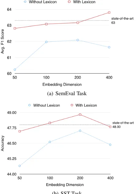
Figure3illustrates the robustness of our lexicon integrated models with respect to the size of word embeddings. Our baseline produces inconsistent and unstable results as different sizes of word em-beddings are used. Furthermore, a larger size of word embeddings tends to significantly outperform a smaller size of word embeddings. Such tendency is reduced with the incorporation of lexicon em-beddings. While the standard deviations for the accuracies achieved by the baseline using different sizes of word embeddings are 0.8491 and 1.1909 for S16 and SST, respectively, they are reduced to 0.4208 and 0.5764 respectively for lexicon inte-grated models. Furthermore, the accuracy achieved by the lexicon integrated model using the word em-bedding size 50 is higher or equal to the highest

accuracy achieved by the baseline using the word embedding size 200, which implies that it is pos-sible to build more compact models using lexicon embeddings without compromising accuracy.

(a) SemEval Task

(b) SST Task

4.4 Analysis

4.4.1 Randomness in Deep Learning

Different random seeds when training the CNN models could possibly change the behavior of mod-els, sometimes by more than 1%. This is due to the randomness in deep learning, such as the random shuffling the datasets, initialization of the weights and drop-out rate of a tensor. To reduce the im-pact of random seed on our result and capture the general characteristic of the model, we performed a group analysis by training each model with 10 different random seeds (Figure4).

(a) SemEval Task: The baseline model has a higher variance than the proposed models. Adding lexicon information im-proves the baseline model to be more accurate. In addition, EAV marginally pushes the performance.

(b) SST Task: The baseline model itself is stable because the vocabulary of the word embedding covers approximately all words in SST, as shown in Table3. Although adding lexicon information destabilize the model lightly, lexicon information enhance the accuracy. EAV is advantageous in general. This effect is visually shown in this figure, when comparing naive concatenation (NC; (Section3.2.1) with NC-EAV.

Figure 4: Generalized performance evaluation of the models. Each model is trained 10 times with different random seeds and the results are summa-rized as a bar plot. In this plot, the central red line indicates the median, and the bottom and top edges of the box indicate the 25th and 75th percentiles, respectively. the ’+’ symbol represents outliers.

4.4.2 S16: SemEval’16 Task 4

For S16, the lexicon integration tends to reduce the variances, and the introducing embedding at-tention vectors pushes the accuracy even higher than the models without it across different ran-dom seeds. Another notable observation for S16 is that although multichannel method underperforms when the random seed is fixed to a specific num-ber as seen in Table4, it produces a competitive output in the group analysis setting. Such low per-formance with a fixed random seed is probably at-tributed to the well known problem of optimization, trapping in local optima.

4.4.3 SST: Stanford Sentiment Treebank

The problem conditions for SST are different in terms of vocabulary coverage. This difference is caused by the source of the lexicon embeddings, where all of them were constructed from Twitter dataset. Since most of the lexical words are from Twitter, it shows less vocabulary coverage on SST than that of S16 as shown in the right columns of Table3. Because of this poor relatedness be-tween lexicons and datasets, we hypothesized that adding a lexicon might be less effective on the per-formance of SST task. However, our models seems to successfully adopt exogenous features enough to push the accuracy marginally higher than the models without lexicons.

On the contrary, the coverage of word embed-dings on SST is notably high at around 98%, while only around 70% for S16 (left columns of Table3). These conditions are well reflected in the group analysis of the model in SST. Since word embed-dings themselves are sufficient enough to cover majority of words, the model variance of the base-line is relatively small compared to S16.

4.4.4 Attention

Embedding attention vectors allow to visualize the importance of each word and lexicon for sentiment analysis through a heatmap. In Figure5, all neg-ative words get higher weights (reds), while non-sentimental words do not (greens and light blues) in EAV. This visualization is especially useful for neu-ral models because it provides an compelling ex-planatory information about how the models work.

4.4.5 Learning Speed

is @ 57/59 of scotlands MPs oppose trident , yet

GeorgeOsborne Faslane tomorrow . get urarses down there . 100bn is gon na bspent renewing it

Cream day Day ? Is the calendar trying to kill

National Ice on Sunday and now it ‘s National Hot Dog me ???

did n’t Json Aldean concert #maybenexttime

If I have training tomorrow id be sick and at the

1971 - the Balmoral Furniture Building and Killed four [LINK] 11 December An IRA bomb attack on the Shankill Road destroyed

be hanged oppose it by following a black day

Yakub should to death tomorrow the Mumbai ‘s culprid else will

-1 -0.5 0 0.5 1

Figure 5: Five selected negative tweets with the attention heatmap. Examples are from the set where the baseline gives wrong answers but SC-EAV predicts correctly. Intensity of each word roughly ranges from -1 to 1. This weights (intensities) are the values of the attention vector of the word embeddings in the SC-EAV model. While negative words get more attention (reds), non-sentimental words such as stop words get less attention (greens and light blues).

if lexicon information is incorporated along with EAV. This statement is general behavior because the learning curves in Figure Figure6are the result of averaging ten different learning attempts with different random seeds.

Figure 6: Lexicon information and EAV accelerate the learning speed. High F1 score can be achieved in the earlier step, if lexicon information is incor-porated along with EAV.

5 Conclusion

This paper proposes several approaches that effec-tively integrate lexicon embeddings and an atten-tion mechanism to a well-explored deep learning framework, Convolutional Neural Networks, for sentiment analysis. Our experiments show that lexi-con integration can improve accuracy, stability, and efficiency of the traditional CNN model. Multiple training results with different random seeds show the generalization of the effectiveness of using lex-icon embeddings and embedding attention vectors. The training curve comparison further shows an-other benefit of this integration for more robust learning. The attention heatmap analysis confirms that embedding attention vectors endow CNN mod-els with explanatory features, which gives good understanding of how the CNN models work.

Much more future work is left. The proposed at-tention models are applied to each single word. However, focusing on multiple words could give more promising information. Application of the attention mechanism to multiple words at the same time is a possible direction. Majority of the lex-icons in this work are from tweet dataset. More lexicon dataset from general could be used to im-prove the coverage of our system. We focused on a simple and yet well performing system. In order to maximize the score, ensemble of multi layer CNN models could be applied.5

Acknowledgments

We gratefully acknowledge the support of the Uni-versity Research Committee Grant (URC) from Emory University, and the Infosys Research En-hancement Grant. Any contents expressed in this material are those of the authors and do not neces-sarily reflect the views of these awards and grants. Special thanks are due to Jung-Hyun Kang for pro-ducing the wonderful figures.

References

Dzmitry Bahdanau, Kyunghyun Cho, and Yoshua Ben-gio. 2014. Neural machine translation by jointly learning to align and translate. ICLR.

Kan Chen, Jiang Wang, Liang-Chieh Chen, Haoyuan Gao, Wei Xu, and Ram Nevatia. 2015. Abc-cnn: An attention based convolutional neural net-work for visual question answering. arXiv preprint arXiv:1511.05960.

Kyunghyun Cho, Bart Van Merri¨enboer, Caglar Gul-cehre, Dzmitry Bahdanau, Fethi Bougares, Holger Schwenk, and Yoshua Bengio. 2014. Learning phrase representations using rnn encoder-decoder for statistical machine translation.EMNLP,. 5_{All our resources are publicly available}

Ronan Collobert, Jason Weston, L´eon Bottou, Michael Karlen, Koray Kavukcuoglu, and Pavel Kuksa. 2011. Natural language processing (almost) from scratch. Journal of Machine Learning Research

12(Aug):2493–2537.

Jan Deriu, Maurice Gonzenbach, Fatih Uzdilli, Au-relien Lucchi, Valeria De Luca, and Martin Jaggi. 2016. Swisscheese at semeval-2016 task 4: Sen-timent classification using an ensemble of convolu-tional neural networks with distant supervision. Pro-ceedings of SemEvalpages 1124–1128.

Xiaowen Ding, Bing Liu, and Philip S Yu. 2008. A holistic lexicon-based approach to opinion mining. InProceedings of the 2008 international conference on web search and data mining. ACM, pages 231– 240.

Ronen Feldman. 2013. Techniques and applications for sentiment analysis. Communications of the ACM

56(4):82–89.

Kevin Gimpel, Nathan Schneider, Brendan O’Connor, Dipanjan Das, Daniel Mills, Jacob Eisenstein, Michael Heilman, Dani Yogatama, Jeffrey Flanigan, and Noah A Smith. 2011. Part-of-speech tagging for twitter: Annotation, features, and experiments. In Proceedings of the 49th Annual Meeting of the Association for Computational Linguistics: Human Language Technologies: short papers-Volume 2. As-sociation for Computational Linguistics, pages 42– 47.

Minqing Hu and Bing Liu. 2004. Mining and summa-rizing customer reviews. InProceedings of the tenth ACM SIGKDD international conference on Knowl-edge discovery and data mining. ACM, pages 168– 177.

Nal Kalchbrenner, Edward Grefenstette, and Phil Blunsom. 2014a. A convolutional neural net-work for modelling sentences. arXiv preprint arXiv:1404.2188.

Nal Kalchbrenner, Edward Grefenstette, and Phil Blunsom. 2014b. A convolutional neural net-work for modelling sentences. In Proceed-ings of the 52nd Annual Meeting of the As-sociation for Computational Linguistics (Volume 1: Long Papers). Association for Computational Linguistics, Baltimore, Maryland, pages 655–665.

http://www.aclweb.org/anthology/P14-1062.

Soo-Min Kim and Eduard Hovy. 2004. Determining the sentiment of opinions. In Proceedings of the 20th international conference on Computational Lin-guistics. Association for Computational Linguistics, page 1367.

Yoon Kim. 2014. Convolutional neural net-works for sentence classification. arXiv preprint arXiv:1408.5882.

Svetlana Kiritchenko, Xiaodan Zhu, and Saif M Mo-hammad. 2014. Sentiment analysis of short infor-mal texts. Journal of Artificial Intelligence Research

50:723–762.

Quoc V. Le and Tomas Mikolov. 2014. Dis-tributed representations of sentences and docu-ments. In Proceedings of the 31th International Conference on Machine Learning, ICML 2014, Bei-jing, China, 21-26 June 2014. pages 1188–1196.

http://jmlr.org/proceedings/papers/v32/le14.html.

Bing Liu. 2012. Sentiment analysis and opinion min-ing. Synthesis lectures on human language technolo-gies5(1):1–167.

Minh-Thang Luong, Hieu Pham, and Christopher D Manning. 2015. Effective approaches to attention-based neural machine translation. EMNLP.

Saif Mohammad, Svetlana Kiritchenko, and Xiaodan Zhu. 2013a. Nrc-canada: Building the state-of-the-art in sentiment analysis of tweets. InProceedings of the seventh international workshop on Seman-tic Evaluation Exercises (SemEval-2013). Atlanta, Georgia, USA.

Saif M Mohammad, Svetlana Kiritchenko, and Xiao-dan Zhu. 2013b. Nrc-canada: Building the state-of-the-art in sentiment analysis of tweets. arXiv preprint arXiv:1308.6242.

Tony Mullen and Nigel Collier. 2004. Sentiment analy-sis using support vector machines with diverse infor-mation sources. InEMNLP. volume 4, pages 412– 418.

Preslav Nakov, Alan Ritter, Sara Rosenthal, Fabrizio Sebastiani, and Veselin Stoyanov. 2016. Semeval-2016 task 4: Sentiment analysis in twitter. In Pro-ceedings of the 10th International Workshop on Se-mantic Evaluation (SemEval-2016). Association for Computational Linguistics, San Diego, California, pages 1–18. http://www.aclweb.org/anthology/S16-1001.

Bo Pang and Lillian Lee. 2005. Seeing stars: Ex-ploiting class relationships for sentiment categoriza-tion with respect to rating scales. InProceedings of the 43rd Annual Meeting on Association for Compu-tational Linguistics. Association for Computational Linguistics, pages 115–124.

Bo Pang and Lillian Lee. 2008. Opinion mining and sentiment analysis. Foundations and trends in infor-mation retrieval2(1-2):1–135.

Mickael Rouvier and Benoit Favre. 2016. Sensei-lif at semeval-2016 task 4: Polarity embedding fusion for robust sentiment analysis. In Proceedings of the 10th International Workshop on Semantic Eval-uation (SemEval-2016). Association for Computa-tional Linguistics, San Diego, California, pages 202– 208. http://www.aclweb.org/anthology/S16-1030. Kevin J Shih, Saurabh Singh, and Derek Hoiem. 2016.

Where to look: Focus regions for visual question an-swering. CVPR.

Richard Socher, Brody Huval, Christopher D Manning, and Andrew Y Ng. 2012. Semantic compositional-ity through recursive matrix-vector spaces. In Pro-ceedings of the 2012 Joint Conference on Empirical Methods in Natural Language Processing and Com-putational Natural Language Learning. Association for Computational Linguistics, pages 1201–1211. Richard Socher, Alex Perelygin, Jean Y Wu, Jason

Chuang, Christopher D Manning, Andrew Y Ng, and Christopher Potts. 2013. Recursive deep models for semantic compositionality over a sentiment tree-bank. InProceedings of the conference on empirical methods in natural language processing (EMNLP). Citeseer, volume 1631, page 1642.

Marijn F Stollenga, Jonathan Masci, Faustino Gomez, and J¨urgen Schmidhuber. 2014. Deep networks with internal selective attention through feedback connec-tions. InAdvances in Neural Information Process-ing Systems. pages 3545–3553.

Maite Taboada, Julian Brooke, Milan Tofiloski, Kim-berly Voll, and Manfred Stede. 2011. Lexicon-based methods for sentiment analysis. Computational lin-guistics37(2):267–307.

Theresa Wilson, Janyce Wiebe, and Paul Hoffmann. 2005. Recognizing contextual polarity in phrase-level sentiment analysis. InProceedings of the con-ference on human language technology and empiri-cal methods in natural language processing. Associ-ation for ComputAssoci-ational Linguistics, pages 347–354. Kelvin Xu, Jimmy Ba, Ryan Kiros, Kyunghyun Cho, Aaron Courville, Ruslan Salakhutdinov, Richard S Zemel, and Yoshua Bengio. 2015. Show, attend and tell: Neural image caption generation with vi-sual attention. International Conference for Ma-chine Learning (ICML).

Toshihiko Yanase, Kohsuke Yanai, Misa Sato, Toshi-nori Miyoshi, and Yoshiki Niwa. 2016. bunji at semeval-2016 task 5: Neural and syntactic models of entity-attribute relationship for aspect-based sen-timent analysis. Proceedings of SemEvalpages 289– 295.

Zichao Yang, Xiaodong He, Jianfeng Gao, Li Deng, and Alex Smola. 2016. Stacked attention networks for image question answering. CVPR.

Wenpeng Yin and Hinrich Sch¨utze. 2014. An explo-ration of embeddings for generalized phrases. In

ACL (Student Research Workshop). pages 41–47.

Wenpeng Yin and Hinrich Sch¨utze. 2015. Multi-channel variable-size convolution for sentence classification. In Proceedings of the Nineteenth Conference on Computational Natural Lan-guage Learning. Association for Computational Linguistics, Beijing, China, pages 204–214.