Topic and audience effects on distinctively Scottish vocabulary usage in Twitter data

Topic and audience effects on distinctively Scottish vocabulary usage

in Twitter data

Philippa Shoemark∗

p.j.shoemark@ed.ac.uk James Kirby

†

j.kirby@ed.ac.uk Sharon Goldwater

∗

sgwater@inf.ed.ac.uk

∗_{School of Informatics} University of Edinburgh

†_{Dept. of Linguistics and English Language} University of Edinburgh

Abstract

Sociolinguistic research suggests that speakers modulate their language style in response to their audience. Similar ef-fects have recently been claimed to occur in the informal written context of Twit-ter, with users choosing less region-specific and non-standard vocabulary when address-ing larger audiences. However, these stud-ies have not carefully controlled for the possible confound of topic: that is, tweets addressed to a broad audience might also tend towards topics that engender a more formal style. In addition, it is not clear to what extent previous results generalize to different samples of users. Using mixed-effects models, we show that audience and topic have independent effects on the rate of distinctively Scottish usage in two demo-graphically distinct Twitter user samples. However, not all effects are consistent be-tween the two groups,underscoring the im-portance of replicating studies on distinct user samples before drawing strong conclu-sions from social media data.

1 Introduction

Linguistic variation in social media is a growing research area, with interest stemming both from the engineering goal of developing tools that work well across different styles and dialects (Hovy, 2015; Stoop and van den Bosch, 2014; Vyas et al., 2014; Huang and Yates, 2014), and from the social sci-ence goal of studying user behaviour (Bamman et al., 2014; Eisenstein, 2015; Huang et al., 2016; Nguyen et al., 2015). However, this type of re-search is often complicated by the messy nature of social media data, which can make it hard to con-trol for different explanatory factors and to know

whether results obtained on a particular user sample generalize to another sample.

For example, previous studies have suggested that Twitter users modulate their use of regional and non-standard language depending on the expected size of the audience (operationalized as whether a Tweet contains hashtags,@-mentions, or neither) (Pavalanathan and Eisenstein, 2015a; Shoemark et al., 2017). However, these studies did not suffi-ciently control for possible effects of topic, which may be confounded with audience size: e.g., users may use more hashtags when discussing political events than when discussing daily routines. These studies also did not look at the degree to which their results generalize across different populations of users.

In this work we study two largely disjoint groups of (mainly) Scottish Twitter users: one group sent tweets geotagged within Scotland, while the other used hashtags related to the 2014 Scottish indepen-dence referendum. We use mixed-effects models to tease apart the effects of audience and topic on their choice of Scottish-specific terms. We find that in both user groups, topic and audience have independent effects on the rate of Scottish usage, providing stronger evidence than in previous work that users are indeed sensitive to their audience.

Nevertheless, our study does not confirm all as-pects of previous work. When comparing our two user groups, the effect of topic is qualitatively sim-ilar: tweets about lifestyle or politics have lower rates of Scottish usage than “chitchat” tweets. How-ever, the effects of audience differ between the two groups. For the geotagged users, rates of Scot-tish usage follow the pattern predicted by previous research: lowest among tweets with the largest expected audience, and rising as the expected au-dience size shrinks. In contrast, the independence referendum group showed a less consistent and less pronounced pattern which does not align cleanly

with audience size. We were unable to find a clear explanation of this difference. Nevertheless, it highlights the difficulty of sampling representative groups from social media data and the need to in-terpret results with caution until they are shown to generalize across several different populations.

2 Background

Bell’s (1984) Audience Design theory posits that intra-speaker stylistic variation is primarily condi-tioned by the audience of the interaction. Bell argues that stylistic variation across topics de-rives from so-called ‘reference groups’ whom the speaker associates with the topics in question, and predicts that effects of topic on style variation will be weaker than direct effects of audience. However, later studies of spoken conversation (e.g. Rickford and McNair-Knox, 1994) have suggested that both topic and audience affect a speaker’s style, and that topic may even have a greater effect. Topic also appears to influence stylistic variation in computer-mediated communication—for example, statistical associations between lexical features and author attributes such as gender are often mediated by the topic of discourse (Herring and Paolillo, 2006; Bamman et al., 2014).

Our work is primarily inspired by two previous studies of Twitter users and how their use of re-gional lexical variants is influenced by either au-dience (Pavalanathan and Eisenstein, 2015a) or topic (Shoemark et al., 2017). In the first of these, Pavalanathan and Eisenstein (2015a) studied lexi-cal items that were strongly associated with tweets from specific regions of the US, as determined by a data-driven approach (Eisenstein et al., 2011). They found that users were less likely to use these regional terms, as well as other nonstandard terms, in tweets containing hashtags, and more likely to do so in tweets containing@-mentions (i.e., other users’ IDs). They attributed these findings to style-shifting in relation to audience size, since tweets with hashtags are more likely to be viewed by users outside of the author’s follower group, while by de-fault tweets which begin with a mention are shown only to the author, the mentioned user, and their mutual followers.

While suggestive, there are alternative explana-tions for this finding. For example, in their study of Scottish tweets, Shoemark et al. (2017) pointed out that if users use the word ‘masel’ (a Scottish vari-ant of standard English ‘myself’) less frequently in

tweets with hashtags, it could be simply because people talk about themselves less in tweets with hashtags, not because they are modulating the use of a regionally specific variant.

Shoemark et al. (2017) focused mainly on ef-fects of topic rather than audience, but to avoid similar confounds, they measured the frequencies of regional variants of lexical variables1_relativeto their standard variants. They found that, amongst users who tweeted about the Scottish indepen-dence referendum, both pro- and anti-indepenindepen-dence users decreased their use of Scottish-specific terms in tweets containing referendum-related hashtags, compared to other tweets. A follow-up analysis suggested that this effect might be due to the larger audience obtained by using referendum-related hashtags, but the evidence was indirect as the origi-nal study was not designed to test that hypothesis.

Our work extends these two previous studies by building models that include factors for both topic and audience. We follow Shoemark et al. (2017) in focusing on variables that alternate between Scot-tish English and Standard English variants, but use a wider range of topics identified with a topic model rather than just hashtags. We use mixed-effects logistic regression in order to establish whether there are independent effects of audience and topic, whilst controlling for variation in the base rate of Scottish-variant usage across different users and variables. In addition, we explicitly examine how different methods of sampling users might affect results, by performing the same study on two user groups gathered in different ways.

3 Data

3.1 Lexical variables

We use 50 of the 51 lexical variables identified by Shoemark et al. (2017). Each variable consists of one or more distinctively Scottish variants and one or more Standard English variants, all of which are referentially and syntactically equivalent; examples are shown in Table 1. From the original 51 vari-ables, we discardSHIT, since the variant identified

as Scottish-specifc,SHITE, is used at a higher rate

than the Scottish-specific forms of the other vari-ables (e.g. 27% ofSHIToccurences in Shoemark et

al.’s Indyref-Tweets dataset are realized asSHITE;

Variable Scottish variants Std variants DONT DEH,DINI,DINNY DONT,DO NOT

FOOTBALL FITBA FOOTBALL

MYSELF MASEL,MASELF MYSELF

SOMETHING SUHIN SOMETHING

TO TAE TO,TOO

Table 1: Examples of lexical variables.

onlyvariable for which any Scottish variant use is observed. This suggests thatSHITEis less marked

as ‘distinctively Scottish’ than the Scottish-specific variants of the other 50 variables.

3.2 Dataset construction

We aim to study Scottish language use, but only a small proportion of Twitter users disclose their location, either by including it in their user profile or by opting to automatically tag their tweets with geographic coordinates when using a GPS-enabled device. Moreover, studies have indicated that those who do share their location are not representative of the wider Twitter user base (Pavalanathan and Eisenstein, 2015b; Sloan and Morgan, 2015).

To help assess the generalizability of our find-ings, we therefore consider two datasets, both covering the same time period but sampled from distinct (though slightly overlapping) populations: ‘Scottish Geotag Users’, who have tagged their

tweets with locations in Scotland; and ‘Indyref Hashtag Users’, who have used hashtags relating to the 2014 Scottish Independence Referendum. As we will demonstrate, users in the two samples do differ in some aspects of their behaviour, empha-sizing how biases implicit in the construction of datasets can affect results.

Our two groups of users are taken from the Geotagged-Scotland (GS) and Indyref-Tweets (IT) datasets collected by Shoemark et al. (2017). Both of these datasets were drawn from an archive of Twitter’s ‘Spritzer’ stream, which provides a 1% sample of the public data flowing through Twit-ter, covering the period from September 2013 to September 2014. The GS dataset consists of tweets by users for whom the archive contained at least one tweet which was geotagged with a location in Scotland, while the IT dataset consists of users for whom it contained at least one tweet with a hashtag relating to the 2014 Scottish Independence referen-dum (see Table 3 in Shoemark et al. (2017) for a list of hashtags).

As a heuristic to filter out bots and spammers,

IH Users SG Users

(a) N Users 14,572 17,942 N Tweets 4,703,040 1,750,343 N Variables 10,482,683 3,733,133

% Scottish 0.5 1.8

(b) N Users 12,101 11,307 N Tweets 4,674,251 1,678,498 N Variables 10,424,067 3,594,659

% Scottish 0.5 1.8

(c) N Users 10,786 10,103 N Tweets 3,456,277 1,371,694 N Variables 7,689,621 2,878,352

% Scottish 0.7 2.3

(d) N Users 10,784 10,103 N Tweets 2,165,320 1,112,931 N Variables 4,934,186 2,365,496

% Scottish 0.8 2.3

Table 2: Dataset statistics for Indyref Hashtag Users and Scottish Geotag Users (a) after basic pre-processing, (b) after discarding users with<50 vari-able instances, (c) after discarding users for which there is strong evidence of non-use of Scottish vari-ants and (d) after labelling audience & topic. ‘% Scottish’ is the percentage of variables realized as the Scottish variant.

we computed the proportion of tweets for each user in the GS and IT datasets which contained URLs, and discarded users for whom this proportion was in the 90th percentile. For the remaining users, we then retrieved a more complete set of their tweets: for each user we attempted to retrieve all the tweets they posted in August, September, or October 2014 (excluding retweets), using Twitter’s REST API. The API allows us to retrieve up to 3200 of a user’s most recent tweets, so if a user had posted more than 3200 tweets since autumn 2014, we were un-able to retrieve their tweet histories for this period. We obtained complete histories for at least one of the three months for a total of 18,370 Scottish Geo-tag (SG) Users, and 14,832 Indyref HashGeo-tag (IH) Users. We then applied some simple ad-hoc text filters to remove tweets produced by apps which au-tomatically share user’s horoscopes or track users’ follower counts, as well as some particularly preva-lent types of marketing tweets. See Table 2a for summary statistics after this filtering step. Note that there are 363 users who are in both datasets.

Scot-tish variants.

Finally, since our population of interest is those who vary between Scottish and standard variants, we discard individuals for whom we had enough observed variable instances to conclude that they probablyneverused distinctively Scottish variants of any of our variables. For SG Users, we chose the threshold of ‘enough observed variable instances’ to be 298, since this is the smallest valuensuch that the cumulative binomial probability of seeing at least one Scottish variant innvariable instances is≥0.99(assuming a constant usage rate of Scot-tish variants of 0.0184, as listed in Table 2b). That is, if we assume that any user who does use Scot-tish variants will do so 1.84% of the time, then in 99% of cases where we have observed at least 298 variable instances from such a user, we would ex-pect a Scottish variant to have been used in at least one of those instances. For IH Users, we assumed a constant usage rate of distinctively-Scottish vari-ants of 0.05, and discarded all those for whom we had observed at least 870 variable instances and no Scottish variants. Table 2c provides summary statistics for the two resulting datasets.

When considering the differences in average rates of Scottish variant usage across the two groups, it is important to note that Shoemark et al. (2017) identified these Scottish variants using the GS dataset, i.e. the same dataset from which we drew our Scottish Geotag Users. It is therefore to be expected that that the Scottish Geotag Users would use these variants at a higher rate, and it is important to bear in mind that the Indyref Hashtag Users may be more frequent users of other distinc-tively Scottish variants.

4 Topic & Audience

4.1 Audience labelling

We follow Pavalanathan and Eisenstein (2015a) in assuming that tweets containing hashtags (any token prepended with the ‘#’ character) typically have a wider audience than other tweets, since any-one interested in a particular topic or event can browse the stream of Tweets which contain associ-ated hashtags. Conversely, tweets beginning with

@-mentions typically have a narrow audience since by default they only appear in the feeds of the au-thor, the mentionee, and users who follow both the author and the mentionee. Any user @-mentioned in a tweet (whether at the beginning, or elsewhere within the tweet) will by default receive a special

Broadcast @-Init @-Internal Hashtag Multiple 0

5 10 15 20 25 30 35 40 45

%

SG IH

Figure 1: Distribution of tweets with each audience label in the two datasets.

notification drawing their attention to it.

Pavalanathan and Eisenstein hypothesise that both kinds of mention serve to narrow the intended audience, whilst hashtags serve to widen it, relative to broadcast tweets (i.e., those without hashtags or mentions, which appear on the feeds of all the au-thor’s followers). The grounds for hypothesising a narrowing function for tweet-internal mentions are less evident than those for tweet-initial mentions, since tweets which do not begin with a mention are

notlimited by default to the feeds of the author and mentionee’s mutual followers.

We label each variable instance in our two datasets with three binary variables indicating whether or not they contain hashtags, initial men-tions, and/or internal mentions. We then discard any tweets for which two or more of these indica-tors are activated, since we do not have intuitive a priori hypotheses about how combining more than one of these variables within a single tweet would affect its intended audience.

Figure 1 shows the proportion of tweets in each dataset which have each audience label (or which had multiple labels and were subsequently dis-carded), and reveals qualitative differences in the two groups’ behaviour: SG Users post relatively more ‘broadcast’ tweets, whilst IH Users use rela-tively more hashtags (which is unsurprising given that they were selected on the basis of their hashtag use).

4.2 Topic labelling

topics. We use the inferred topic model parameters to label each tweet with a topic, as described below.

The corpus was preprocessed as follows: tweets were tokenised using the Twokenize program2_{, a} tokeniser designed specifically for Twitter text, and all non-alphabetic tokens, except for those which begin with hashtags, were discarded. The vocabu-lary was then pruned to the 100,000 most frequent terms across the two datasets. We set the number of topics,T, to 30, and used symmetric Dirichlet priors ofα= 50

T andβ = 0.01on the multinomial

distributions over topics and terms, respectively3_. The Gibbs sampler was run for 750 iterations.

Upon inspection of the most probable words and documents for each topic, we deemed that twenty of the topics could be grouped into three broader themes, which we describe as ‘chatter’ , ‘lifestyle’ , and ‘politics’ . Later, we consider a different group-ing, where we split off a ‘sports’ theme from the ‘lifestyle’ theme, and an ‘indyref’ theme from the ‘politics’ theme. Table 3 shows the most probable words (excluding stopwords) for each topic within these three/five themes. Of the ten topics that we did not assign to these themes, four could be de-scribed as spam topics, four as foreign language, and two as relating to purely stylistic dimensions as opposed to any particular topic of discussion: one for distinctively Scottish terms, and the other for ‘netspeak’-style spellings and abbreviations.

To assign topic labels to individual tweets, we take a Gibbs sample and then for a given tweet, each topictis assigned a weight, defined as

weight_t= X

w∈w

ˆ p(t|w)

wherew is the bag of words which occur in the tweet (excluding stopwords and any variant of any of our variables of interest), andpˆ(t|w)is obtained by maximum likelihood estimation from the Gibbs-sampled topic-token assignments. Finally, we take the topic with the highest weight, and label the tweet with its broader theme. If the topic with the highest weight is one of the two ‘stylistic’ topics, we defer to the topic with the next highest weight. We discard tweets labelled as ‘spam’ or ‘foreign language’, as well as those for which the highest weight is not unique, if the topics which share this weight belong to different themes.

2_{https://github.com/myleott/ark-twokenize-py}

3_{During development we experimented with values for T} between 10 and 100, andαbetween 0.015 and 1.5, and saw little qualitative difference in the themes that emerged, based on manual inspection of topic keywords.

Chatter Lifestyle Sport Politics Indyref Other Ambiguous 0

5 10 15 20 25 30 35 40 45

%

SG IH

Figure 2: Distribution of tweets with each topic label in the two datasets.

Using this method, we obtain 2.3m broad-topic-labeled variable instances from SG Users, and 4.9m from IH Users. Figure 2 shows the distribution of topics in each data set, and Table 4 gives a break-down of variable instances by audience-type and broad-topic-label. IH Users have a much larger pro-portion of tweets with ‘indyref’ or ‘politics’ labels than SG Users, which once again is unsurprising, given how these users were sampled.

5 Method

We use the glmer() function from the lme4 package (Bates et al., 2015) for R (R Core Team, 2013) to estimate mixed effects logistic regression models, predicting Scottish variant usage (yes = 1, no = 0) from the intended audience size and topic of the tweet in which a lexical variable occurs. Our four-level categorical audience factor (initial mention, internal mention, broadcast, hashtag) is dummy coded into three binary variables, with broadcasts as the reference level. Our tweet topic labels are also dummy coded, taking the ‘chatter’ topic as the reference level. By specifying random effects for users and variables, we control for the influence of different baseline rates of Scottish variant usage across different users and variables. Hence our models are of the form

logit{E(y)}=Xβ+Zu,y∼Bernoulli

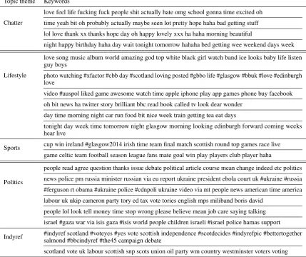
Topic theme Keywords

Chatter

love feel life fucking fuck people shit actually hate omg school gonna time excited oh time yeah bit oh probably actually maybe seen lot pretty hope haha bad getting stuff lol love thank xx thanks hope day oh happy lovely xxx ha haha morning beautiful

night happy birthday haha day wait tonight tomorrow hahaha bed getting wee weekend days week

Lifestyle

love song music album world amazing god top white black girl watch band ice looks baby life listen guy boys

photo watching #xfactor #cbb day #scotland loving posted #gbbo life #glasgow #bbuk #love #edinburgh love

video #auspol liked game awesome watch time apple iphone play app games phone buy facebook oh bit news ha twitter story brilliant bbc read book called tv look dear wonder

day time morning night car run food bit nice week train getting tea eat days

tonight day week time tomorrow night glasgow morning looking edinburgh forward coming weeks hear live

Sports cup win ireland #glasgow2014 irish time team final match scottish round top games race live game celtic team football season league fans mate goal win play players club player haha

Politics

people read agree question thanks issue debate political article course mean change indeed etc politics news police pm russia minister russian via eu report ukraine president ebola court uk #ukraine #russia #ferguson rt obama #ukraine police #cdnpoli ukraine video via mt people news american time america labour uk ukip cameron party tory ed tax vote tories english mps miliband boris david

people lol look tell money time stop wrong please believe mean job care saying talking israel #gaza war via isis gaza #isis world people children israeli #israel police hamas support Indyref #indyref scotland #voteyes #yes vote scottish independence #scotdecides #indyrefpic #bettertogether_{salmond #bbcindyref #the45 campaign debate}

scotland vote uk labour scottish snp scots union oil party wm country westminster voters voting

Table 3: Topic themes and the top 15 keywords for each topic within each theme

Audience Topic Chatter Lifestyle Politics All

(a) Broadcast 598,673 (2.7) 334,143 (2.3) 295,981 (1.8) 1,228,797 (2.4) Initial Mention 352,981 (3.0) 164,909 (2.9) 188,191 (1.9) 706,081 (2.7) Internal Mention 92,682 (1.8) 63,242 (1.5) 56,727 (1.2) 212,651 (1.6) Hashtag 67,630 (1.8) 69,833 (1.4) 80,504 (1.2) 217,967 (1.4) All 1,111,966 (2.7) 632,127 (2.3) 621,403 (1.7) 2,365,496 (2.3)

(b) Broadcast 308,797 (1.3) 341,592 (0.9) 658,520 (0.8) 1,308,909 (1.0) Initial Mention 644,459 (1.1) 394,036 (1.0) 1,026,634 (0.6) 2,065,129 (0.8) Internal Mention 76,403 (0.6) 96,123 (0.5) 203,275 (0.4) 375,801 (0.5) Hashtag 124,333 (0.7) 197,925 (0.5) 862,089 (0.5) 1,184,347 (0.5) All 1,153,992 (1.1) 1,029,676 (0.8) 2,750,518 (0.6) 4,934,186 (0.8)

GRAND

AD

BALLS _SHITTY BIRD ALRIGHT PISSED PISSING

BIRDS

DEFINITEL

Y

DOGS

I

KNO

W

YOURSELF

BALL SORE YOUR OLD MYSELF GIVES

OUT OFF

DO

WN

F

OOTBALL WANT

TO

WITH _DIDNT ISNT GOOD _HOUSE DOING FR

OM

HOME DONT

DOESNT

SOMETHING TOMRR

O

W

ONE OUR DO THING _ABOUT THINK GOING

TO OF

W

AS ON

THA

TS

YOU _HAVE JUST

−5

−4

−3

−2

−10 1 2 3 4

BLUP

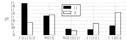
Figure 3: Barplots of by-variable BLUPs for SG Users (black bars) and for IH Users (white bars).

−4 −2 0 2 4 6 8 SG by-user BLUPs 0

5 10 15 20 25 30 35 40

%

−4−2 0 2 4 6 8 10 12 IH by-user BLUPs

Figure 4: Histograms of by-user BLUPs.

6 Results and Discussion

6.1 Random Intercepts

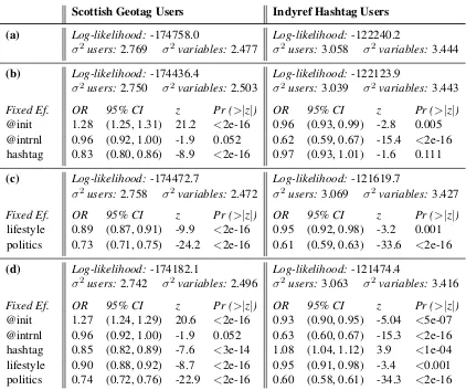
We begin by constructing null models that predict the log odds of choosing a Scottish variant using only intercepts, which we allow to vary randomly by each user and by each lexical variable. The estimated variances of the by-user and by-variable adjustments to the intercept are given in Table 5a, for SG and IH Users, respectively.

The Best Linear Unbiased Predictors (BLUPs) of the by-variable random intercerpts (i.e. the poste-rior estimates, given the data and model parameters, of the adjustment to the intercept for each variable) are shown in Figure 3. In both datasets, open class variables (e.g. GRANDAD,BALLS,DOGS) tend to

have higher rates of Scottish variant usage than closed class variables (e.g.WAS,OF,YOU).

Figure 4 shows the distributions of by-user BLUPs. Although the models assume a normal distribution over the by-user intercepts, the BLUPs are positively skewed. We suspect the BLUPs re-flect the fact that our datasets contain a mixture of two populations: Scottish speakers, who use Scot-tish variants at a range of rates, and non-ScotScot-tish speakers, who rarely if ever use Scottish variants. The non-Scottish speakers are responsible for the large number of users with slightly negative inter-cepts. Unfortunately there is no straightforward way to separate these groups (especially for users

with a relatively small number of observations). However, users with a constant near-zero rate of Scottish variant usage should, at worst, dilute any true effects of topic or audience on rates of usage, but should not change the direction of those effects.

6.2 Random Intercepts + Audience Effects

We now check whether Pavalanathan and Eisen-stein’s (2015a) reported effects of hashtags and mentions on the odds of using regional variants in US tweets, are replicated for distinctively Scottish variants in our two datasets.

We augment our null models with our dummy-coded audience factors as fixed effects. For each dataset, we assess the goodness-of-fit using chi-square tests on the log-likelihoods. Compared to the null models with only random effects, including fixed effects for audience significantly improves the fit on both datasets (SG:χ2(3) = 643.05, p =

<2.2e-16; IH:χ2(3) = 232.69, p =<2.2e-16). Parameters of the models with Audience effects are in Table 5b. Our results for SG Users largely accord with those of Pavalanathan and Eisenstein (2015a): Scottish variants are positively associated with tweet-initial mentions, and negatively associ-ated with hashtags. Relative to broadcast tweets, the odds of seeing Scottish variants are about 28% higher in tweets with initial mentions, and about 17% lower in tweets with hashtags. However, while Pavalanathan and Eisenstein also found an associa-tion between the use of tweet-internal menassocia-tions and local/non-standard words in their data, our model does not show such a relationship in the SG dataset.

IH Users, initial mentions arenegativelyassociated with Scottish variants, though the effect size is very small. Internal mentions are also negatively asso-ciated with Scottish variants, and in this case the effect is relatively large (in contrast with SG Users, for whom we found no effect). We discuss possible reasons for this result in Section 6.4.

6.3 Random Intercepts + Topic Effects

Next, we test for a relationship between the topic of a tweet and the odds of Scottish variant usage. For both datasets, models with fixed effects for topic significantly improve the fit over random-effects-only models (SG:χ2(2) = 570.48, p =<2.2e-16; IH:χ2(2) = 1241, p =<2.2e-16).

Parameters of the models are in Table 5c. The ef-fects of tweet topic are qualitatively similar in each dataset: relative to ‘chatter’ tweets, tweeting about the ‘lifestyle’ topic reduces the odds of choosing Scottish variants by 11% for SG Users and 5% for IH Users, while tweeting about politics reduces them by 27% for SG Users, and 39% for IH Users.

6.4 Full Models

For each dataset, including fixed effects for audi-ence and topic together significantly improves the model fit, both over the models with fixed effects for audience only (SG Users:χ2(2) = 508.67, p =

<2.2e-16; IH Users: χ2(2) = 1298.9, p =< 2.2e-16), and over the models with fixed effects for topic only (SG:χ2(3) = 581.25, p =<2.2e-16; IH:χ2(3) = 290.6, p =<2.2e-16).

Parameters of the full models are in Table 5d. When fixed effects for audience and topic are in-cluded together in the SG model, their effect sizes barely change. These results suggest that for SG Users, audience and topic have independent effects on Scottish usage, and that even after accounting for topic, the effects of audience size are as pre-dicted by Pavalanathan and Eisenstein (2015a).

In the full IH model, while most of the fixed effect sizes are relatively unchanged, a positive as-sociation between the use of hashtags and Scottish variants emerges. Thus, the model reveals that the qualitative behavior of these users is very different from that of the SG Users. Although topic and au-dience are both significant factors in the models for each group, initial mentions and hashtags have the opposite effects for IH Users as for SG Users (and for Pavalanathan and Eisenstein’s user sample).

Although they primarily interpret their findings in terms of audience size, Pavalanathan and

Eisen-stein acknowledge that mentions and hashtags can affect the composition of the audience in more nu-anced ways than just its size. As an alternative explanation for the positive associations they found between mentions and local/non-standard words, they suggest that authors may use such words to express particular identities or stake claims to local authenticity, specifically when addressing users for whom such claims are meaningful.

In theory, this account could also apply to the positive association we find in the IH dataset be-tweenhashtags and local variants: while on the one hand, the indexing function of hashtags can be conceived of as broadening the audience of a tweet, on the other hand it could serve to narrow the tweet’s intended audience, by explicitly target-ing it at a circumscribed community. Hence, when using hashtags associated with communities for whom the notion of Scottish identity has strong currency (e.g. people with strong views on indyref, or supporters of a particular sports team), IH Users may use Scottish variants initiatively, in order to emphasise that part of their identity.

Suppose that authors tended to decrease their use of Scottish variants when discussing most po-litical issues, but increase it when discussing Scot-tish independence—either to emphasise their own Scottish identity, or to accommodate towards an audience which is likely to contain many Scottish people. If this were the case, our models would be unable to account for this variation directly, since we have grouped indyref and other political issues together. However, since a large proportion (55%) of IH Users hashtag tweets are actually about in-dyref, one way the IH model could account for a difference between indyref and general politics is to increase the weight for hashtags. If this were the case, then including ‘indyref’ as a distinct topic should improve the model fit and alleviate the im-pact on the audience weights. To test this hypothe-sis, we performed a follow-up study where we split the topics into finer-grained categories.

6.5 Finer-grained topics

We added two topic categories, ‘sport’ and ‘in-dyref’, which we split off from the ‘lifestyle’ and ‘politics’ categories, respectively (see Table 3).

Scottish Geotag Users Indyref Hashtag Users (a) Log-likelihood:-174758.0 Log-likelihood: -122240.2

σ2 _{users:2.769 σ}2_{variables:2.477 σ}2_{users:3.058 σ}2 _{variables:3.444} (b) Log-likelihood:-174436.4 Log-likelihood: -122123.9

σ2 _{users:2.750 σ}2_{variables:2.503 σ}2_{users:3.039 σ}2 _{variables:3.443}

Fixed Ef. OR 95% CI z Pr (>|z|) OR 95% CI z Pr (>|z|)

@init 1.28 (1.25, 1.31) 21.2 <2e-16 0.96 (0.93, 0.99) -2.8 0.005 @intrnl 0.96 (0.92, 1.00) -1.9 0.052 0.62 (0.59, 0.67) -15.4 <2e-16

hashtag 0.83 (0.80, 0.86) -8.9 <2e-16 0.97 (0.93, 1.01) -1.6 0.111

(c) Log-likelihood:-174472.7 Log-likelihood: -121619.7

σ2 _{users:2.758 σ}2_{variables:2.472 σ}2_{users:3.069 σ}2 _{variables:3.427}

Fixed Ef. OR 95% CI z Pr (>|z|) OR 95% CI z Pr (>|z|)

lifestyle 0.89 (0.87, 0.91) -9.9 <2e-16 0.95 (0.92, 0.98) -3.2 0.001 politics 0.73 (0.71, 0.75) -24.2 <2e-16 0.61 (0.59, 0.63) -33.6 <2e-16

(d) Log-likelihood:-174182.1 Log-likelihood: -121474.4

σ2 _{users:2.742 σ}2_{variables:2.496 σ}2_{users:3.063 σ}2 _{variables:3.416}

Fixed Ef. OR 95% CI z Pr (>|z|) OR 95% CI z Pr (>|z|)

@init 1.27 (1.24, 1.29) 20.6 <2e-16 0.93 (0.90, 0.95) -5.04 <5e-07 @intrnl 0.96 (0.92, 1.00) -1.9 0.052 0.63 (0.60, 0.67) -15.3 <2e-16 hashtag 0.85 (0.82, 0.89) -7.6 <3e-14 1.08 (1.04, 1.12) 3.9 <1e-04 lifestyle 0.90 (0.88, 0.92) -8.7 <2e-16 0.95 (0.91, 0.98) -3.4 <0.001 politics 0.74 (0.72, 0.76) -22.9 <2e-16 0.60 (0.58, 0.61) -34.3 <2e-16

Table 5: Summary of model parameters for the two datasets: (a) random intercepts only, (b) random intercepts + audience effects, (c) random intercepts + topic effects, (d) full model. σ2 _{usersand σ}2

variablesare variance estimates for the random intercepts.Fixed Ef.tables show odds ratios (OR) derived from logit coefficients, with roughly estimated confidence intervals (using approximate standard errors), and results of Wald’s z-tests.

for IH Users (c.f. Table 5d).

In general, the effect sizes and directions of the newly defined subtopics are similar to those of the broad topics from which they were isolated, and more importantly, changing the topic definitions has no effect on the audience coefficients for either user group. This provides some evidence that our results are not highly sensitive to the precise choice of topics.

7 Conclusion

This study examined how Twitter users shift their use of Scottish variants depending on the topic and audience. We looked at two groups of users with different overall rates of Scottish usage and found that both topic and audience affect usage in both groups. The qualitative effects of topic were sim-ilar across the two groups, demonstrating a clear

Acknowledgments

This work was supported in part by the EPSRC Cen-tre for Doctoral Training in Data Science, funded by the UK Engineering and Physical Sciences Re-search Council (grant EP/L016427/1) and the Uni-versity of Edinburgh.

References

David Bamman, Jacob Eisenstein, and Tyler Schnoebe-len. 2014. Gender identity and lexical variation in

social media.Journal of Sociolinguistics18(2):135–

160.

Douglas Bates, Martin M¨achler, Ben Bolker, and Steve Walker. 2015. Fitting linear mixed-effects models

using lme4. Journal of Statistical Software67(1):1–

48.

Allan Bell. 1984. Language style as audience design. Language in society13(02):145–204.

David M Blei, Andrew Y Ng, and Michael I Jordan.

2003. Latent dirichlet allocation. Journal of

Ma-chine Learning Research3(Jan):993–1022.

Jacob Eisenstein. 2015. Systematic patterning

in phonologically-motivated orthographic variation. Journal of Sociolinguistics19(2):161–188.

Jacob Eisenstein, Amr Ahmed, and Eric P. Xing. 2011.

Sparse additive generative models of text. In

Pro-ceedings of the International Conference on Ma-chine Learning. pages 1041–1048.

Thomas L Griffiths and Mark Steyvers. 2004.

Find-ing scientific topics. Proceedings of the National

Academy of Sciences101(suppl 1):5228–5235.

Susan C Herring and John C Paolillo. 2006. Gender

and genre variation in weblogs. Journal of

Sociolin-guistics10(4):439–459.

Liangjie Hong and Brian D Davison. 2010. Empirical

study of topic modeling in twitter. InProceedings of

the first workshop on social media analytics. ACM, pages 80–88.

Dirk Hovy. 2015. Demographic factors improve

classi-fication performance. InProceedings of the 53rd

An-nual Meeting of the Association for Computational Linguistics. Association for Computational Linguis-tics, pages 752–762.

Fei Huang and Alexander Yates. 2014. Improving word alignment using linguistic code switching data. In Proceedings of the 14th Conference of the Euro-pean Chapter of the Association for Computational Linguistics. Association for Computational Linguis-tics, Gothenburg, Sweden, pages 1–9.

Yuan Huang, Diansheng Guo, Alice Kasakoff, and Jack Grieve. 2016. Understanding U.S. regional

linguis-tic variation with Twitter data analysis. Computers,

Environment and Urban Systems59:244 – 255. Dong Nguyen, Dolf Trieschnigg, and Leonie Cornips.

2015. Audience and the use of minority languages

on twitter. InProceedings of the Ninth International

Conference on Web and Social Media. pages 666– 669.

Umashanthi Pavalanathan and Jacob Eisenstein. 2015a. Audience-modulated variation in online social me-dia. American Speech90(2):187–213.

Umashanthi Pavalanathan and Jacob Eisenstein. 2015b. Confounds and consequences in geotagged Twitter

data. In Proceedings of the 2015 Conference on

Empirical Methods in Natural Language Processing. Association for Computational Linguistics, pages 2138–2148.

R Core Team. 2013. R: A Language and Environment

for Statistical Computing. R Foundation for Sta-tistical Computing, Vienna, Austria. http://www.R-project.org/.

John R Rickford and Faye McNair-Knox. 1994. Addressee-and topic-influenced style shift: A

quanti-tative sociolinguistic study. Sociolinguistic

perspec-tives on registerpages 235–276.

Philippa Shoemark, Debnil Sur, Luke Shrimpton, Iain Murray, and Sharon Goldwater. 2017. Aye or naw, whit dae ye hink? Scottish independence and

lin-guistic identity on social media. InProceedings of

the 15th Conference of the European Chapter of the Association for Computational Linguistics: Volume 1, Long Papers. Association for Computational Lin-guistics, pages 1239–1248.

Luke Sloan and Jeffrey Morgan. 2015. Who tweets with their location? Understanding the relationship between demographic characteristics and the use of

geoservices and geotagging on Twitter. PloS one

10(11):e0142209.

Wessel Stoop and Antal van den Bosch. 2014. Using idiolects and sociolects to improve word prediction. InProceedings of the 14th Conference of the Euro-pean Chapter of the Association for Computational Linguistics. Association for Computational Linguis-tics, Gothenburg, Sweden, pages 318–327.