GPU-Friendly Local Regression for Voice Conversion
Taylor Berg-Kirkpatrick Dan Klein Computer Science Division
University of California, Berkeley {tberg,klein}@cs.berkeley.edu
Abstract
Voice conversion is the task of transforming a source speaker’s voice so that it sounds like a target speaker’s voice. We present a GPU-friendly local regression model for voice con-version that is capable of converting speech in real-time and achieves state-of-the-art ac-curacy on this task. Our model uses a new approximation for computing local regression coefficients that is explicitly designed to pre-serve memory locality. As a result, our infer-ence procedure is amenable to efficient imple-mentation on the GPU. Our approach is more than 10X faster than a highly optimized CPU-based implementation, and is able to convert speech 2.7X faster than real-time.
1 Introduction
Voice conversion is the task of transforming an ut-terance from a source speaker’s voice into a target speaker’s voice. The primary setup in recent work has been to learn this transformation from a paral-lel corpus consisting of recordings of the same se-quence of sentences read by both source and tar-get speakers (Stylianou et al., 1998). The converted speech is evaluated by how well its spectral proper-ties match those of the target voice.
While various models have been proposed (Stylianou et al., 1998; Toda et al., 2007; Toda et al., 2005), the most accurate ones are non-parametric because the mapping between two voices’ spectra can be highly non-linear (Helander et al., 2012; Popa et al., 2012). Unfortunately, while non-parametric methods are accurate, they are also slow – current non-parametric approaches to voice conversion are too compute-intensive for the real-time speed re-quired by many voice conversion applications. In this paper, we begin with the state-of-the-art local
linear regression (LLR) model used by by Popa et al. (2012) for voice conversion, and present a new GPU-based inference approach that greatly acceler-ates it, to much faster than real-time.
LLR, in principle, requires each new model pre-diction to be a function of the entire set of training examples. In practice, LLR depends most strongly on nearby points, so a standard CPU implementa-tion will skip distant points, with limited loss of ac-curacy. A GPU cannot exploit sparsity in the same way (scan and skip) without suffering from memory bottlenecks, but even a GPU will be relatively slow if all training points are included in each computation. Our primary algorithmic change is to make use of a new sparsity structure that allows the GPU to skip major sections of the training data while still using dense memory access patterns on the points it does process. In experiments, this inference technique is more than 10X faster than a highly-optimized CPU-based implementation, operates almost three times faster than real-time, and is only slightly less accu-rate than the CPU-based method.
2 Background and Model
Most representations of speech that are useful for speech processing break the acoustic signal into sep-arate components that represent the sound source (the lungs and vocal folds) and sound filter (the vo-cal tract) portions of the vovo-cal apparatus. Work on voice conversion is generally focused on transform-ing the representation of the vocal tract. We follow this approach and learn a transformation of a mel-cepstral representation of the acoustic signal (Kawa-hara, 2006).
We treat the task as a multiple regression prob-lem. In order to produce the transformed signal, we break the source signal into a sequence of frames, each of which is a 24-dimensional vector of
cepstral coefficients. We denote a single frame of input mel-cepstral coefficients as x. In order to produce the transformed signal, we simply predict frame-by-frame. Specifically, for a frame x of the input we predict a transformed frameyˆas the mode of densityp(y|x), which we estimate from training data. A naive approach would be to use a linear model:
y=Ax+
Here, is a Gaussian noise term, and the model is parameterized by the transformation matrix,A. For now, we assume training data are already frame-aligned (see Section 4). Let yi be frame i of the
target signal in the training data. Similarly, let xi
be the corresponding frame of the source signal in the training data. Thus, using this linear model, we would estimate the transformation as:
ˆ
A=argmin
A
X
i
kyi−Axik2
This very simple approach works, to some extent, but, because it cannot capture important non-linear relationships betweenxandy, it is far from state-of-the-art. A more popular approach is to use a Gaus-sian mixture model (GMM) to jointly generate both source and target cepstral features (Stylianou et al., 1998; Toda et al., 2007; Toda et al., 2005). This approach essentially learns different linear transfor-mations for different regions of the input space, cap-turing some non-linearity. However, the GMM in-troduces a new problem: the posterior over the la-tent clusters learned by the GMM can be highly peaked (Popa et al., 2012) and as a result distortion is introduced by discontinuities at cluster boundaries. Thus, we adopt neither the simple linear approach nor the GMM. We instead the state-of-the-art fully non-parametric approach introduced by Popa et al. (2012). This method, described in the next section, learns transformations that capture non-linearity but vary smoothly as the input changes.
2.1 Local Regression
Like Popa et al. (2012), we use local linear regres-sion (LLR) (Cleveland, 1979) to estimate p(y|x). LLR is a non-parametric method that estimates
p(y|x) as a linear transformation that varies slowly
with the inputx. Specifically,p(y|x)is estimated as follows:
y=A(x)·x+
ˆ
A(x) =argmin
A
X
i
w(x, xi)· kyi−Axik2
The transformationAˆis a function ofx, and is com-puted by solving a weighted least squares problem that depends onx. wis a kernel function that mea-sures similarity between the current input, x, and each of the source training frames, xi. We use a
Gaussian kernel:
w(x, xi) =exp
−kx−xik2
2σ2
Intuitively, for each input framexwe solve a sepa-rate least squares regression where each training da-tum is weighted by its similarity to the input. As the input varies, so will the weighting, and thus so will the linear transformation.
3 Inference
Exact inference using LLR is too computationally expensive for most applications since it means solv-ing a least squares problem over the entire trainsolv-ing set for each input framex. A common approach is to define a neighborhood function that, for each in-put frame x, selects K training frames xi that are
most relevant tox. Then,Aˆ(x)is computed by only solving the least squares problem over this neigh-borhood. This approach can work well in practice since the support for each local least squares prob-lem is relatively sparse. By choosing the right neigh-borhood function, work can be skipped without sub-stantially impacting learning.
3.1 Inference on the CPU
The standard approach when using a CPU is to let the neighborhood function pick out the indices of the
K training frames xi that maximizew(x, xi). We
let this particular neighborhood function be called
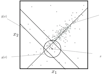
g(x), depicted in Figure 1. Using this approach, for input framex, Aˆ(x) has the following closed form expression:
ˆ
G(x) is a matrix formed by appending the train-ing source vectors in the neighborhood ofx. More specifically,G(x)is a matrix that has the vectorsx>
i
s.t.i∈g(x)as its rows. Similarly,H(x)is a matrix that has the vectorsy>
i s.t. i ∈ g(x)as its rows (in
the corresponding order). W(x)is a matrix that has the weightsw(x, xi)s.t.i∈g(x)along its diagonal
(also in the corresponding order).
This approach is much faster than the exhaustive method, but at typical audio sampling frequencies, inferring the transformation of the signal for an en-tire sentence can take over 30 seconds on a mod-ern CPU, which is too slow for real-time conversion. In order to transform the signal for a new sentence,
ˆ
A(x)must be computed for each frame. This means that for each frame x, the distance to all training source frames must be computed, neighborhood ma-tricesG(x)andH(x)must be formed, followed by several matrix multiplies, an LU decomposition, and a triangular solve operation.
3.2 Inference on the GPU
The computation ofAˆ(x)for a block of multiple in-put frames can be done in parallel if a fixed amount of lag is tolerated in the conversion process. The parallel computation of large number of small dense matrix operations (multiply, LU decomposition, tri-angular solve) is a perfect fit for implementation a GPU, which can achieve vastly more throughput than modern CPUs can. However, using the CPU’s neighborhood structure on the GPU has a crippling bottleneck. The extraction of the neighborhood ma-tricesG(x)andH(x)from the training data requires a large number of memory accesses that are effec-tively random. The indices of the closest K train-ing source vectors to an inputx are generally non-contiguous. As a result, theKvectors in each of the neighborhood matrices must be copied with sepa-rate memory accesses, and since random access time on modern GPUs is very slow, extraction becomes a bottleneck. In initial experiments, we found that when this approach is implemented on a GPU it is even slower than the CPU-based implementation.
In contrast, memory bandwidth is extremely high on modern GPUs. Thus, if it were possible to order the training vectorsxi andyiin GPU memory such
that neighborhood matrices G(x) and H(x) were composed of contiguous blocks of training vectors,
x1
x2
surrogate neighborhood
˜
g(x)
g(x)
neighborhood input framex
first principal direction GPU
[image:3.612.324.531.61.209.2]CPU
Figure 1: Depiction of standard neighborhood functiong(x) used for local regression on the CPU and surrogate neighbor-hood functiong˜(x)used for inference on the GPU, plotted for two-dimensional input data.
extraction on the GPU could be made very effi-cient. Unfortunately, with the current definition of the neighborhood function,g, such an ordering does not exist. Therefore, we define a new GPU-friendly neighborhood function,g˜, for which an ordering that permits contiguous extraction does exist.
Letu(x)be the projection of source vectorxonto the first principal component resulting from running PCA on the source side of the training data. Now, we define˜gas follows: g˜(x)is the set ofK indices for which|u(x)−u(xi)|is the smallest, or, in other
words, the set of training indices with source projec-tions closest to the projection of the input frame. By ordering the training data by their projection onto the first principal component, we can ensure that
G(x)andH(x)are contiguous in memory.
The hope is that this approach yields substantial speedups on the GPU without negatively impacting the learned transformation (see Section 4). Figure 1 depicts the difference between the CPU neighbor-hood functiongand the GPU functiong˜. Intuitively, when most of the variance in the training data occurs along the first principal direction, the CPU and GPU neighborhood functions may be similar since the distance between projections is a good proxy for dis-tance in the original space. The weighting function,
w, is still computed in the original space, so distant training vectors that are inadvertently included in the neighborhood will be severely down-weighted. The potential pitfall is that for a fixed neighborhood size,
˜
System Scottish Male to US Female US Female to Scottish MaleCD Time Frac. RT CD Time Frac. RT
GMM 7.05 1.1 3.7X 7.01 0.7 3.9X
CPU LLR 5.99 12.2 0.3X 6.51 8.75 0.3X
GPU LLR 5.98 1.4 2.7X 6.55 0.9 2.9X
Table 1: Voice conversion results for the GMM baseline system, CPU-based local linear regression baseline system, and the GPU-based local linear regression method. The cepstral distortion (CD), average inference time per sentence in seconds (Time), and fraction of real-time (Frac. RT) are shown. Smaller cepstral distortion corresponds to more accurate transformations and fractions of real-time that exceed one imply faster than real-time operation.
4 Experiments
We run a series of experiments to determine whether our GPU-based inference technique offers speeds-ups and at what cost to accuracy.
Baselines We compare our LLR-based conversion
system that performs inference on the GPU (using the GPU-friendly neighborhood function) with two different baseline systems. The first baseline sys-tem also uses LLR, but performs inference on the CPU using the standard neighborhood function. The second baseline is the GMM model of Toda et al. (2007), which is known to be fast and is widely used in practice. The size, K, of both CPU and GPU neighborhoods was set on a development data to the smallest value that did not show degraded perfor-mance compared to exact local regression.
Implementation We implemented our
GPU-based LLR technique using the CUDA API (Nickolls et al., 2008), and the CUBLAS API which contains bindings for GPU BLAS routines. We ran the system using an NVIDIA Tesla K40c GPU. We built a multi-threaded implementation of CPU-based inference for local regression using calls to CPU BLAS routines, and ran this system on a 4.4GHz 4-core Intel CPU.
Data We train and test on a portion of the CMU Arctic database. The training data consists of 70 sentences spoken by both a US female speaker and a Scottish male speaker. The testing data consists of 20 sentences spoken by the same two speakers. We give results for converting in both directions, from the female voice to the male voice, and from the male voice to the female voice.
Frame Alignment Since the source and target
speakers speak at slightly different rates, our train-ing data consist of different numbers of frames for each training sentence. We use dynamic time warp-ing to induce the frame alignment. Specifically, we find the minimum cost monotonic alignment from source frames into target frames where the cost of each alignment edge is the L2 distance between the corresponding vectors. We use a distortion limit of 2, and a linear distortion cost.
Analysis and Synthesis We use the CMU
imple-mentation of the STRAIGHT analysis and synthe-sis methods introduced by Kawahara (2006). This is the same method used many state-of-the-art voice conversion systems, included our GMM baseline of Toda et al. (2007). We transform the top 24 cep-stral coefficients using our system, but process the power coefficient and fundamental frequency sep-arately, using simple transformations for the latter two components.
Evaluation In order to evaluate the accuracy of
our model we measure the cepstral distortion be-tween the predicted ceptstral framesyˆand the actual cepstral frames for the target voicey. The cepstral distortion is calculated as follows:
distortion(ˆy, y)∝ kyˆ−yk
We using dynamic time warping to align the pre-dicted frame sequence to the target frame sequence.
4.1 Results
GMM baseline in terms of average cepstral distor-tion. The GMM baseline, is however, the fastest of the compared systems. For both experiments, it is able to produce transformations substantially faster than real-time. The CPU-based local regres-sion baseline achieves the best overall cepstral dis-tortion, but is also the slowest method. In both ex-periments, it operates at 0.3X real-time speed. The GPU-based local regression method performs only slightly worse overall than the exact method in terms of cepstral distortion, yet in both experiments it op-erates substantially faster than real-time, nearly as fast as the parametric baseline.
5 Conclusion
We have demonstrated a method for substantially speeding-up inference using a non-parametric es-timator for spectral voice conversion. Related approaches may prove useful for making non-parametric estimators more efficient in other areas of speech and language processing.
Acknowledgements
This work was partially supported by BBN un-der DARPA contract HR0011-12-C-0014 and by an NSF fellowship for the first author. Thanks to the anonymous reviewers for their insightful comments. We further gratefully acknowledge a hardware do-nation by NVIDIA Corporation.
References
William S Cleveland. 1979. Robust locally weighted regression and smoothing scatterplots. Journal of the American statistical association, 74(368):829–836. E. Helander, H. Silen, T. Virtanen, and M. Gabbouj.
2012. Voice conversion using dynamic kernel partial least squares regression. IEEE transactions on audio, speech, and language processing, 20(3):806–817. H. Kawahara. 2006. Straight, exploitation of the other
aspect of vocoder: Perceptually isomorphic decompo-sition of speech sounds. Acoustical science and tech-nology, 27(6):349–353.
John Nickolls, Ian Buck, Michael Garland, and Kevin Skadron. 2008. Scalable parallel programming with cuda. Queue, 6(2):40–53.
Victor Popa, Hanna Silen, Jani Nurminen, and Moncef Gabbouj. 2012. Local linear transformation for voice
conversion. InAcoustics, Speech and Signal Process-ing (ICASSP), 2012 IEEE International Conference on, pages 4517–4520. IEEE.
Yannis Stylianou, Olivier Cappé, and Eric Moulines. 1998. Continuous probabilistic transform for voice conversion. Speech and Audio Processing, IEEE Transactions on, 6(2):131–142.
Tomoki Toda, Alan W Black, and Keiichi Tokuda. 2005. Spectral conversion based on maximum likelihood es-timation considering global variance of converted pa-rameter. InICASSP (1), pages 9–12.