Proceedings of NAACL-HLT 2018, pages 541–550
Learning Domain Representation for Multi-Domain Sentiment
Classification
Qi Liu1, Yue Zhang1 and Jiangming Liu2
Singapore University of Technology and Design, Singapore1
University of Edinburgh, UK2
{qi liu, yue zhang}@sutd.edu.sg
Abstract
Training data for sentiment analysis are abun-dant in multiple domains, yet scarce for other domains. It is useful to leveraging data avail-able for all existing domains to enhance per-formance on different domains. We investigate this problem by learning domain-specific rep-resentations of input sentences using neural network. In particular, a descriptor vector is learned for representing each domain, which is used to map adversarially trained domain-general Bi-LSTM input representations into domain-specific representations. Based on this model, we further expand the input representa-tion with exemplary domain knowledge, col-lected by attending over a memory network of domain training data. Results show that our model outperforms existing methods on multi-domain sentiment analysis significantly, giv-ing the best accuracies on two different bench-marks.
1 Introduction
Sentiment analysis has received constant research
attention due to its importance to business (Pang
et al.,2002;Hu and Liu,2004;Choi and Cardie, 2008; Socher et al., 2012; Vo and Zhang, 2015; Tang et al.,2014). For multiple domains, such as movies, restaurants and digital products, manu-ally annotated datasets have been made available. A useful research question is how to leverage
re-sources available across all domains to improve
sentiment classification ona certaindomain.
One naive domain-agnostic baseline is to com-bine all training data, ignoring domain differ-ences. However, domain knowledge is one valu-able source of information availvalu-able. To utilize
this, there has been recent work ondomain-aware
models via multi-task learning (Liu et al., 2016;
Nam and Han,2016), building an output layer for each domain while sharing a representation net-work. Given an input sentence and a specific test
domain, the output layer of the test domain is cho-sen for calculating the output.
These methods have been shown to improve over the naive domain-agnostic baseline. How-ever, a limitation is that outputs for different do-mains are constructed using the same domain-agnostic input representation, which leads to weak utilization of domain knowledge. For different do-mains, sentiment words can differ. For example, the word “beast” can be a positive indicator of camera quality, but irrelevant to restaurants or movies. Also, “easy” is frequently used in the elec-tronics domain to express positive sentiment (e.g. the camera is easy to use), while expressing nega-tive sentiment in the movie domain (e.g. the end-ing of this movie is easy to guess).
We address this issue by investigating a model that learns domain-specific input representations for multi-domain sentiment analysis. In particular, given an input sentence, our model first uses a bi-directional LSTM to learn a general sentence-level representation. For better utilizing data from all
domains, we use adversarial training (Ganin and
Lempitsky,2015;Goodfellow et al.,2014) on the Bi-LSTM representation.
The general sentence representation is then mapped into a domain-specific representation by attention over the input sentence using
explic-itly learneddomain descriptors, so that the most
salient parts of the input are selected for the spe-cific domain for sentiment classification. Some
ex-amples are shown in Figure 2, where our model
pays attention to word “engaging” for movie re-views, but not for laptops, restaurants or cameras. Similarly, the word “beast” receives attention for laptops and cameras, but not for restaurants or movies.
In addition to the domain descriptors, we further introduce a memory network for explicitly
repre-senting domain knowledge. Here domain
I am satisfied with this camera Sequence:
Embedding Layer Lookup:
Bi-LSTM: Average Pooling: Softmax:
𝑦"
(a)Mix: shared parameters for all domains.
I am satisfied with this camera
Sequence:
Embedding Layer
Lookup: Bi-LSTM: Average Pooling: Softmax:
𝑦"1
𝑦"2
…… 𝑦"𝑚
(b) Multi: shared input representations and domain-specific prediction layers.
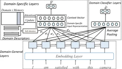
Domain i Memory
Update
Self-Attention Attention
I am satisfied with this camera Embedding Layer
𝑦"𝑖
Domain-General Layers
Context Vector Domain-Specific Input Representation
… Domain Descriptors
Domain-Specific Layers Domain Classifier Layers
ai 1ai2 ai3 ai
4 ai5
ai6 Average
Pooling
𝑑%𝑖
[image:2.595.78.285.365.482.2](c) Our model: domain knowledge is better utilized by do-main descriptors, memories and adversarial training.
Figure 1: Models.
edge refers to example training data in a specific domain, which can offer useful background con-text. For example, given a sentence ‘Keep cool if you think it’s a wonderful life will be a heart-warming tale about life like finding nemo’, algo-rithms can mistakenly classify it as positive based on ‘wonderful’ and ‘heartwarming’, ignoring the fact that ‘it’s a wonderful life’ is a movie. In this case, necessary domain knowledge revealed in other sentences, such as ‘The last few minutes of the movie: it’s a wonderful life don’t cancel out all the misery the movie contained’ is helpful. Given a domain-specific input representation, we make attention over the domain knowledge memory net-work to obtain a background context vector, which is used in conjunction with the input
representa-tion for sentiment classificarepresenta-tion.
Results on two real-world datasets show that our model outperforms the aforementioned multi-task learning methods for domain-aware training, and also generalizes to unseen domains. Our code is
released1.
2 Problem Definition
Formally, we assume the existence ofmsentiment
datasets {Di}mi=1, each being drawn from a
do-main i. Di contains |Di| data points (sij, di, yji),
where sij is a sequence of words w1, w2...w|si
j|,
each being drawn from a vocabulary V, yi
j
in-dicates the sentiment label (e.g. yi
j ∈ {−1,+1}
for binary sentiment classification) anddi is a
do-main indicator (since we use 1 to m to number
each domain,di = i). The task is to learn a
func-tion f which maps each input (sij, di) to its
cor-responding sentiment label yji. The challenge of
the task lies in how to improve the
generaliza-tion performance of mapping funcgeneraliza-tionf both
in-domain and cross-in-domain by exploring the corre-lations between different domains.
3 Baselines
3.1 Domain-Agnostic Model
One naive baseline solution ignores the domain
characteristics when learning f. It simply
com-bines the datasets{Di}mi=1 into one and learns a
single mapping functionf. We refer to this
base-line asMix, which is depicted in Figure1(a).
Given an input sij, its word sequence
w1, w2...w|si
j| is fed into a word embedding
layer to obtain embedding vectors x1, x2...x|si
j|.
The word embedding layer is parameterized by an
embedding matrixEw ∈RK×|V|, whereKis the
embedding dimension.
Bidirectional LSTM: To acquire a
seman-tic representation of input sij, a bidirectional
extension (Graves and Schmidhuber, 2005) of
Long Short-Term Memory (LSTM) (Hochreiter
and Schmidhuber, 1997) is applied to capture sentence-level semantics both left-to-right and right-to-left. As a result, two sequences of
hid-den states are obtained, hid-denoted as h1,
h2...
h|si
j|
andh1, h2...h|si
j|, respectively. We concatenate
ht
1https://github.com/leuchine/
andhtat each time step to obtain the hidden states h1, h2...h|si
j|, which are of sizes2K.
Output Layer: Average pooling (Boureau et al., 2010) is applied on the hidden states
h1, h2...h|si
j| to obtain an input representation I
i j
forsij,
Iji =
P|si
j|
t=1ht
|si
j|
(1)
Finally, softmax is applied over Ii
j to obtain
a probability distribution of all sentiment labels. During training, cross entropy is used as loss
function, denoted asL(f(si
j), yij) for data points
(si
j, di, yij), and AdaGrad (Duchi et al., 2011) is
applied to update parameters.
3.2 Multi-Domain Training
We build a second baseline for domain-aware sentiment analysis. A state-of-the-art architecture (Liu et al., 2016; Nam and Han, 2016) is used
as depicted in Figure 1 (b), where m mapping
functions fi are learned for each domain. Given
the input representationIi
jobtained in Equation1,
multi-task learning is conducted, where each do-main has a dodo-main-specific set of parameters for softmax to predict sentiment labels with shared input representation layers. The input domain
in-dicator di instructs which set of softmax
param-eters to use here and each domain has its own cross entropy lossLi(fi(sji, di), yij)for data points
(sij, di, yij). We denote this baseline asMulti.
4 Method
4.1 Domain-Aware Input Representation
The above baseline Multi achieves
state-of-the-art performance for multi-domain sentiment
anal-ysis (Liu et al., 2016), yet the domain
indica-tor di is used solely to select softmax
parame-ters. As a result, domain knowledge is hidden and
under-utilized. Similar toMix andMulti, we use
a Bi-LSTM to learn representations shared across domains. However, we introduce domain-specific layers to better capture domain characteristics as
shown in Figure1(c).
Different domains have their own sentiment lex-icons and domain differences largely lie in which words are relatively more important for deciding the sentiment signals. We use the neural
atten-tion mechanism (Bahdanau et al., 2014) to select
words, obtaining domain-specific input represen-tations.
In our model, domain descriptors are
intro-duced to explicitly capture domain characteristics,
which are parametrized by a matrixN ∈R2K×m.
Each domain descriptor corresponds to one
col-umn ofN and has a length of2K, the same as the
bidirectional LSTM hidden statesht. This matrix
is automatically learned during training.
Given an input (si
j, di), we apply an
embed-ding layer and Bi-LSTM to generate its
domain-general representationh1, h2, ..., h|si
j|and use the
corresponding domain descriptor Ni to weigh
h1, h2, ..., h|si
j| for obtaining a domain-specific
representation. To this end, there are two most commonly used attention mechanisms: additive
attention (Bahdanau et al., 2014) and dot
prod-uct attention (Ashish Vaswani,2017). We choose
additive attention here, which utilizes a feed-forward network with a single hidden layer, since it achieves better accuracies in our development.
The input representation Ii
j becomes a weighted
sum of hidden states:
Iji =
|si
j|
X
t=1
aijtht s.t. |si
j|
X
t=1
aijt= 1 (2)
The weightaijt reflects the similarity between the
domaini’s descriptorNi and the hidden stateht.
aijtis evaluated as:
lijt=vTtanh(P Ni+Qht)
aijt= exp(l
i
jt)
P|si
j|
p=1exp(ljpi )
(3)
HereP ∈R4K×2K,Q∈ R4K×2K andv ∈R4K
are parameters of additive attention.P andQ
lin-early projectNi andht to a hidden layer,
respec-tively. The projected space is set as 4K
empiri-cally, since we find it beneficial to project the
vec-tors into a larger layer.vserves as the output layer.
Softmax is applied to normalizelijt. We name this
method DSRfor learning domain-specific
repre-sentations.
4.2 Self-Attention over Domain Descriptors
DSR uses a single domain descriptor to attend
‘restaurant’). To model the interaction between domains, a self-attention layer is applied using dot product attention empirically, as shown in Figure 1(c):
Ninew=N softmax(NTNi) (4)
We compute dot products betweenNi and every
domain descriptors. The dot products are
normal-ized using the softmax function, and Ninew is a
weighted sum of all domain descriptors.Ninewis
used to attend over hidden states, employing
Equa-tion2and3. During back propagation training,
do-main descriptors of similar dodo-mains could be
up-dated simultaneously. We name this method
DSR-sa, which denotes domain-specific representation
with self-attention.
4.3 Explicit Domain Knowledge
To further capture domain characteristics, we
de-vise a memory network (Weston et al., 2014;
Sukhbaatar et al.,2015;Kumar et al.,2016) frame-work to explicitly represent domain knowledge. Our memory networks hold example training data of a specific domain for retrieving context data during predictions.
Formally, we use a memory Mi ∈ R2K×|Di|
(|Di|is the total number of training instances of
domaini) to hold domain-specific representations
Iji of training instances for the domaini.
Memory Network: We directly setIjias thejth
column of the memoryMi. Formally,
Mji =Iji (5)
Obtaining A Context Vector Using Back-ground Knowledge: Given an input Ii
j, we
gen-erate a context vectorCjito support predictions by
memory reading:
Cji =Misoftmax((Mi)TIji) (6)
Dot product attention is applied here, which is faster and more space-efficient than additive at-tention, since it can be implemented using highly optimized matrix multiplication. Dot products are
performed betweenIi
jand each column ofMiand
the scores are normalized using the softmax func-tion. The final context vector is a weighted sum of
Mi’s columns.
Output: We concatenate the context vector and the domain-specific input representation, feed-ing the result to softmax layers. Similar to the
baseline Multi, each domain has its own loss
Li(fi(sij, di), yij). We name this method as
DSR-ctxfor context vector enhancements.
Reducing Memory Size: In the naive
imple-mentation, the memory size|Mi|is equal to the
to-tal number of saved sequences, which can be very large in practice. We explore two ways to reduce memory size.
(1) Organizing memory by the vocabulary. We
set |Mi| = |V|, where each memory column of
Micorresponds to a word in the vocabulary.
Dur-ing memory writDur-ing, Iji updates all the columns
that correspond to the words w in its input
se-quencesij by exponential moving average:
Mwi =decay∗Mwi + (1−decay)Iji
In this way, two input representations update the same column of the memory network if and only if they share at least one common word.
(2) Fixing the memory size by clustering.|Mi|
is set to a fixed size andIji only updates the
mem-ory column that is most similar toIji, i.e.Iji only
update the columnarg max(Mi)TIi
j. In this way,
semantically similar inputs are clustered and up-date the same column.
4.4 Adversarial Training
We use embeddings and Bi-LSTM, parametrized
by θdg, to generate domain-general
represen-tations. However, the distributions of domain-general representations for all domains can be
dif-ferent (Goodfellow et al., 2014), which
contami-nates the representations (Liu et al.,2017) and
im-poses negative effects for in-domain predictions. For cross-domain testing, the discrepancies cause domain shift, which harms prediction accuracies
on target domains (Ganin and Lempitsky, 2015).
Thus, models that can generate domain-invariant representations for all domains are favorable for utilizing multi-domain datasets.
We incorporate adversarial training to enhance the domain-general representations. As shown in
Figure 1 (c), domain classifier layers are
intro-duced, parametrized by θdc, which predicts how
likely the input sequence si
j comes from each
domain i. We denote its cross entropy loss as
Lat(fat(sij), di) for data points (sij, di, yji) from
domaini(note that we usedi as its label instead
of input here).
lay-ers, the model is trained by a minimax game.
For dataset Di drawn from domain i, we
mini-mize its loss Li(fi(sji, di), yji) for sentiment
pre-dictions, while maximizing the domain classifier lossLat(fat(sij), di), controlled byλ:
min
θdg,θds
X
Di
Li(fi(sij, di), yij)−λLat(fat(sij), di),
(7)
whereθdsis the set of domain-specific parameters
including domain descriptors, attention weights
and softmax parameters. We fix θdc and update
θdg and θds here. Its adversarial part maximizes
the loss by updatingθdc, while fixingθdgandθds.
max
θdc
X
Di
Li(fi(sij, di), yij)−λLat(fat(sij), di)
(8)
Equations7and8are performed iteratively to
gen-erate domain-invariant representations. We name
this methodDSR-at.
5 Experiments
We evaluate the effectiveness of the model both in-domain and cross-in-domain. The former refers to the setting where the domain of the test data falls into
one of themtraining data domains, and the latter
refers to the setting where the test data comes from one unknown domain.
5.1 Experimental Settings
We conduct experiments on two benchmark datasets. The datasets are balanced, so we use ac-curacy as the evaluation metric in the experiments.
The dataset1contains four domains. The
statis-tics are shown in Table1 , which also shows the
accuracies using baseline methodMixtrained and
tested on each domain. Camera2 consists of
re-views with respect to digital products such as
cam-eras and MP3 players (Hu and Liu, 2004).
Lap-top and Restaurant are laptop and restaurant re-views, respectively, obtained from SemEval 2015
Task 123. Movie4 are movie reviews provided by
Pang and Lee (2004).
The dataset 2 is Blitzer’s multi-domain
senti-ment dataset (Blitzer et al.,2007), which contains
2http://www.cs.uic.edu/˜liub/FBS/
sentiment-analysis.html
3Since the original dataset targets aspect-level sentiment analysis, we remove the sentences with opposite polarities on different aspects. The remaining sentences are labeled with the unambiguous polarity.
4https://www.cs.cornell.edu/people/
pabo/movie-review-data/
Domain Instance Vocab Size Accuracy
Camera (CR) 3770 5340 0.802
Laptop (LT) 1907 2837 0.871
Restaurant (RT) 1572 2930 0.783
Movie (M) 10662 18765 0.773
Table 1: Dataset1statistics.
product reviews taken from Amazon.com, includ-ing 25 product types (domains) such as books, beauty and music. More statistics can be found at
its official website5.
Given each dataset, we randomly select 80%, 10% and 10% of the instances as training, devel-opment and testing sets, respectively.
5.2 Baselines and Hyperparameters
In addition to theMixbaseline, theMultibaseline
(Liu et al., 2016) and our domain-aware models, DSR,DSR-sa,DSR-ctx,DSR-at, we also experi-ment with the following baselines:
MTRL(Zhang and Yeung,2012) is a state-of-the-art multi-task learning method with discrete features. The method models covariances between task classifiers, and in turn the covariances regu-larize task-specific parameters. The feature
extrac-tion forMTRLfollows (Blitzer et al.,2007). We
use this baseline to demonstrate the effectiveness of dense features generated by neural models.
MDA (Chen et al., 2012) is a cross-domain baseline, which utilizes marginalized de-noising auto-encoders to learn a shared hidden represen-tation by reconstructing pivot features from cor-rupted inputs.
FEMA(Yang and Eisenstein,2015) is a cross-domain baseline, which utilizes techniques from neural language models to directly learn feature embeddings and is more robust to domain shift.
NDA(Kim et al.,2016) is a cross-domain
base-line, which usesm+ 1LSTMs, where one LSTM
captures global information across allmdomains
and the remaining m LSTM capture
domain-specific information.
We set the size of word embeddingsK to300,
which are initialized using the word2vec model6
on news. To obtain the best performance, the parameters are set using grid search based on development results. The dropout ratio is
cho-sen from [0.3, ,1]. Learning rate is chosen from
5https://www.cs.jhu.edu/˜mdredze/
datasets/sentiment/
6https://code.google.com/archive/p/
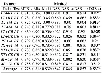
Dataset Method
Train Test MTRL Mix Multi DSR DSR-sa DSR-ctx DSR-at
LT+RT LT 0.817 0.896 0.90 0.908 0.911 0.914 0.92*
LT+RT RT 0.781 0.820 0.85 0.860 0.859 0.863 0.883*
LT+M LT 0.825 0.882 0.90 0.887 0.90 0.904 0.913*
LT+M M 0.743 0.778 0.772 0.788 0.79 0.803 0.811*
LT+CR LT 0.869 0.904 0.906 0.921 0.915 0.92 0.925
LT+CR CR0.774 0.800 0.802 0.822 0.826 0.832 0.844*
RT+M RT 0.792 0.830 0.833 0.853 0.86 0.883 0.9*
RT+M M 0.729 0.765 0.785 0.795 0.801 0.816 0.83*
RT+CR RT 0.783 0.828 0.822 0.847 0.851 0.878 0.887*
RT+CR CR 0.756 0.804 0.814 0.812 0.817 0.831 0.84*
M+CR M 0.745 0.775 0.788 0.798 0.802 0.830 0.839*
M+CR CR 0.758 0.799 0.8110.819 0.812 0.817 0.812
[image:6.595.93.271.62.188.2]Average 0.778 0.818 0.832 0.842 0.845 0.857 0.867*
Table 2: Results using two training domains on dataset
1. * denotesp < 0.01VS. the second best using
Mc-Nemar’s test.
[0.0001,0.001, ,1]. The vocabulary size is
cho-sen from [6000,8000, ,16000]. The batch size
is chosen from [10, ,100]. λ is chosen from
[0.0001,0.001, ,1]. As a result, the mini-batch
size, the size of the vocabulary V, dropout rate,
learning rate for AdaGra and λ for adversarial
training are set to50,10000,0.4,0.5and0.1,
re-spectively. Also, gradient clipping (Pascanu et al.,
2013) is adopted to prevent gradient exploding
and vanishing during training process. Since all datasets only have thousands of instances, we set memory network sizes as training instance sizes in the experiments.
5.3 Working with Known Domains
In this section, we perform in-domain validations. We first combine two datasets for training and test on each domain’s hold-out testing dataset. The
re-sults on dataset1are shown in Table2(the results
on Blitzer’s dataset exhibit similar results and are omitted due to space constraints).
The accuracies of MTRL are significantly
lower than the neural models, which demonstrates the effectiveness of dense features over discrete
features. The baseline Mix improves the average
accuracy from 0.778 to 0.818, and most
multi-domain training accuracies are better compared
to single-domain training in Table 1. Mix
sim-ply combines the two datasets for trainings and ignores domain characteristics, yet improves over single dataset training. This demonstrates that more data reduces over-fitting and leads to
bet-ter generalization capabilities. Multi further
im-proves the average accuracy by1.4%, which
con-firms the effectiveness of utilizing domain infor-mation.
Among our models,DSRfurther improves the
accuracy over Multi by 1%, which confirms the
effectiveness of domain-specific input
representa-tions in multi-domain sentiment analysis.DSR-sa
slightly outperformsDSRby0.03%. Adopting an
additional self-attention layer,DSR-satrains
simi-lar domain descriptors together, thus better model-ing domain relations, which will be further studied
in Section 5.5.2. DSR-ctx outperforms DSR-sa
by 1.2%, which demonstrates the effectiveness of memory networks in utilizing domain-specific
ex-ample knowledge.DSR-atgives significantly the
best results, confirming that domain-invariant rep-resentations achieved by adversarial training in-deed benefit in-domain training. The results are significant using McNeymar’s test.
The results combining all the 4 domains and the 25 domains of the two datasets are shown in the ‘In
domain’ sections of Table3 and Table4,
respec-tively. Here the models are trained using all do-mains’ training data, and tested on each domain’s hold-out test data. Similar patterns are observed
as in Table 2 and DSR-at achieves significantly
the best accuracies (0.867 and 0.907 for the two datasets, respectively).
5.4 Working with Unknown New Domains We validate the algorithms cross-domain. For
dataset 1, models are trained on three domains,
yet validated and tested on the other domain. For
dataset 2, models are trained on 24 domains, yet
validated and tested on the 25th.
SinceDSR-athasmoutputs (one for each
train-ing domain), we adopt an ensemble approach to obtain a single output for unknown test domains. In particular, since the domain classifier outputs probabilities on how likely the test data come from each training domain, we use these probabilities as
weights to average themoutputs.
For NDA,Multi,DSRandDSR-saand
DSR-ctx, we use average pooling to combine them
out-puts. SinceMDAandFEMAare devised to train
on a single source domain, we combine the
train-ing data ofmdomains for training.
The results are shown in the ‘Cross domain’
section of Table3and Table 4, respectively. One
observation is that cross-domain accuracies are worse than in-domain accuracies, showing chal-lenges in unknown-domain testing.
Contrast between our models andFEMA/NDA
In domain Cross domain
Dataset MTRL Mix Multi DSR DSR-sa DSR-ctx DSR-at MTRL Mix MDA Multi FEMA NDA DSR DSR-sa DSR-ctx DSR-at
LT 0.813 0.831 0.900 0.897 0.902 0.898 0.915* 0.763 0.792 0.801 0.808 0.811 0.816 0.822 0.823 0.854 0.878*
RT 0.776 0.801 0.825 0.841 0.845 0.855 0.870* 0.772 0.786 0.789 0.779 0.774 0.776 0.78 0.784 0.814 0.847*
M 0.800 0.803 0.783 0.807 0.812 0.820 0.828* 0.616 0.636 0.642 0.668 0.679 0.684 0.692 0.695 0.725 0.729
CR 0.775 0.786 0.819 0.825 0.828 0.836 0.854* 0.714 0.721 0.736 0.735 0.741 0.745 0.751 0.753 0.789 0.809*
[image:7.595.89.505.68.124.2]Average 0.791 0.805 0.832 0.843 0.847 0.852 0.867* 0.716 0.734 0.742 0.748 0.751 0.755 0.761 0.764 0.796 0.815*
Table 3: In-domain learning and cross-domain results on dataset1. * denotesp <0.01VS. the second best.
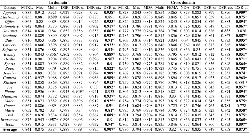
In domain Cross domain
Dataset MTRL Mix Multi DSR DSR-sa DSR-ctx DSR-at MTRL Mix MDA Multi FEMA NDA DSR DSR-sa DSR-ctx DSR-at
Apparel 0.883 0.912 0.921 0.927 0.928 0.92 0.938* 0.828 0.843 0.863 0.854 0.865 0.873 0.882 0.899 0.896 0.909*
Electronics 0.853 0.881 0.899 0.884 0.879 0.883 0.891 0.804 0.826 0.836 0.849 0.845 0.834 0.857 0.859 0.861 0.875*
Office 0.863 0.88 0.89 0.903 0.914 0.925 0.933* 0.824 0.825 0.818 0.824 0.843 0.839 0.854 0.876 0.883 0.894*
Automotive 0.842 0.864 0.873 0.886 0.891 0.902 0.917* 0.791 0.786 0.791 0.797 0.816 0.826 0.835 0.847 0.857 0.867*
Gourmet 0.814 0.838 0.84 0.852 0.856 0.858 0.863* 0.777 0.775 0.764 0.784 0.796 0.803 0.814 0.826 0.832 0.828
Outdoor 0.853 0.889 0.899 0.903 0.907 0.915 0.927* 0.785 0.796 0.805 0.815 0.836 0.829 0.856 0.861 0.867 0.887*
Baby 0.816 0.853 0.86 0.875 0.877 0.892 0.91* 0.803 0.816 0.814 0.821 0.834 0.84 0.845 0.878 0.873 0.895*
Grocery 0.862 0.886 0.898 0.907 0.911 0.917 0.933* 0.806 0.817 0.826 0.846 0.846 0.862 0.88 0.873 0.865 0.886*
Software 0.851 0.876 0.88 0.893 0.898 0.904 0.92* 0.795 0.811 0.816 0.836 0.845 0.836 0.85 0.862 0.884 0.897*
Beauty 0.816 0.843 0.8567 0.862 0.867 0.864 0.889* 0.756 0.768 0.775 0.785 0.795 0.804 0.812 0.812 0.838 0.851*
Health 0.871 0.901 0.904 0.896 0.897 0.896 0.907 0.785 0.807 0.819 0.832 0.845 0.848 0.843 0.834 0.857 0.871*
Sports 0.851 0.883 0.899 0.889 0.882 0.895 0.9 0.759 0.768 0.775 0.784 0.816 0.819 0.821 0.836 0.848 0.864*
Book 0.743 0.803 0.79 0.804 0.809 0.815 0.822* 0.694 0.705 0.716 0.723 0.745 0.743 0.751 0.758 0.779 0.798*
Jewelry 0.816 0.891 0.881 0.893 0.891 0.894 0.909* 0.762 0.769 0.774 0.785 0.795 0.808 0.815 0.835 0.857 0.874*
Camera 0.912 0.937 0.968 0.966 0.959 0.968 0.989* 0.869 0.878 0.886 0.896 0.894 0.908 0.917 0.925 0.942 0.963*
Kitchen 0.815 0.858 0.863 0.875 0.887 0.894 0.913* 0.759 0.768 0.775 0.776 0.794 0.818 0.826 0.856 0.865 0.884*
Toy 0.823 0.863 0.875 0.881 0.884 0.88 0.892* 0.814 0.824 0.815 0.803 0.813 0.832 0.826 0.843 0.845 0.857*
Phone 0.879 0.936 0.94 0.943 0.949* 0.941 0.933 0.805 0.813 0.808 0.818 0.821 0.833 0.836 0.856 0.874 0.894*
Magazine 0.835 0.874 0.872 0.883 0.895 0.917 0.937* 0.805 0.819 0.817 0.816 0.83 0.841 0.845 0.857 0.871 0.896*
Video 0.851 0.873 0.882 0.891 0.896 0.912 0.925* 0.754 0.774 0.794 0.795 0.815 0.822 0.834 0.845 0.855 0.875*
Games 0.867 0.886 0.89 0.883 0.886 0.887 0.9* 0.681 0.684 0.708 0.718 0.723 0.734 0.746 0.765 0.781 0.778
Music 0.752 0.782 0.8 0.798 0.8 0.798 0.81* 0.775 0.769 0.779 0.784 0.795 0.824 0.815 0.823 0.842 0.858*
Dvd 0.795 0.826 0.834 0.847 0.854 0.867 0.889* 0.801 0.794 0.804 0.794 0.814 0.827 0.835 0.845 0.851 0.875*
Instrument 0.873 0.9430.957* 0.896 0.906 0.898 0.9 0.814 0.805 0.813 0.815 0.825 0.836 0.833 0.835 0.845 0.865*
Tools 0.887 0.915 0.931 0.928 0.93 0.932 0.94* 0.805 0.814 0.828 0.835 0.846 0.857 0.864 0.866 0.873 0.897*
Average 0.841 0.875 0.884 0.887 0.89 0.895 0.907* 0.786 0.794 0.801 0.807 0.82 0.827 0.835 0.847 0.858 0.873*
Table 4: In-domain learning and cross-domain results on dataset2. * denotesp <0.01VS. the second best.
NDAalso considered domain-specific
representa-tions. On the other hand, it duplicates the full set of model parameters for each domain, yet
underper-formsDSRandDSR-sa, which records only one
domain descriptor vector for each domain. The contrast shows the advantages of learning domain descriptors explicitly in terms of both efficiency and accuracy.
Similar to the known domain results,
DST-sa and DSR-ctx further improve upon DSR and DSR-sa, showing the effectiveness of do-main memory and adversarial learning. On both
datasets, DSR-at achieves significantly the best
performances, which shows the advantages of domain-invariant representations for unknown-domain testing.
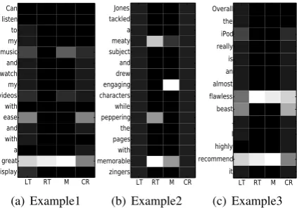
5.5 Case Study 5.5.1 Input Attention
To obtain a better understanding of input attention with domain descriptors, we examine the attention weights of inputs and three examples are displayed
in Figure2, where the x axis denotes the four
do-mains from the first dataset and the y axis shows the words.
In Figure2(a), the domain-specific word ‘ease’
is only selected for the domainsLTandCR, while
the domain-independent word ‘great’ is salient in
all domains. Similarly, in Figure2(b), ‘meaty’ and
‘engaging’ are only salient inRT andM,
respec-tively. In Figure 2 (c), the domain-specific word
‘beast’ is chosen inLTandCR.
These confirm the effectiveness of input
at-tention and DSR-ctx has the capability to pick
out sentiment lexicons in conformity with domain characteristics.
5.5.2 Domain Descriptors
With the self-attention layer, one interesting ques-tion is whether learned domain descriptors can re-flect domain similarities/dissimilarities.
We take out the twenty-five domain descriptors for Blitzer’s dataset and calculate the cosine sim-ilarities between each pair. Also, we calculate the cosine similarities of twenty-five domains based on unigram and bigram representations for ground truth. Pearson correlation coefficient is used to measure the correlations between two sets of
co-sine values. The final score is0.796, which shows
[image:7.595.87.512.152.379.2]LT RT M CR displaygreat
a withand easewith videosmy watchand musicmy to listenCan
0.320.400.480.560.640.720.800.880.96
(a) Example1
LT RT M CR zingers
memorablewith pagesthe pepperingwhile charactersengaging drewand subjectmeaty a tackledJones
0.400.480.560.640.720.800.880.96
(b) Example2
LT RT M CR it
recommendhighly I . beast flawlessalmost anis reallyiPod the Overall
0.320.400.480.560.640.720.800.880.96
[image:8.595.78.291.66.214.2](c) Example3 Figure 2: Attention values (0: black, 1: white).
5.5.3 Memory Network Attention
We further study the attention of memory net-works by randomly picking instances in the test sets and listing the context instances with the greatest attention weights obtained from Equation
6. The results of three test instances and their
con-text instances are shown in Table .
One observation is that semantically similar in-stances are selected to provide extra knowledge for predictions (e.g. a1, a2, b3, c1, c2, c3). An-other observation is that the sentiment polarities between test instances and selected context in-stances are usually the same. We conclude that the memory networks are capable of selecting instruc-tive instances for facilitating predictions.
6 Related Work
Domain Adaptation (Blitzer et al., 2007; Titov, 2011; Yu and Jiang, 2015) adapts classifiers trained on a source domain to an unseen target domain. One stream of work focuses on learn-ing a general representation for different domains based on the co-occurrences of domain-specific
and domain-independent features (Blitzer et al.,
2007;Pan et al.,2011;Yu and Jiang,2015;Yang et al., 2017). Another stream of work tries to identify domain-specific words to improve
cross-domain classification (Bollegala et al., 2011; Li
et al., 2012; Zhang et al., 2014;Qiu and Zhang,
2015). Different from previous work, we utilize
multiplesource domains for cross-domain valida-tion, which makes our method more general and domain-aware.
Multi-domain Learning jointly learn multiple domains to improve generalization. One strand of
work (Dredze and Crammer, 2008; Saha et al.,
2011; Zhang and Yeung, 2012) uses
covari-This place blew me away. By far my new favorite restaurant on the upper-east side.
(a1) This is one of my favorite spot, very relaxing. The food is great all the times. Celebrated my engagement and my wedding here. It was very well organized.
(a2) This is one of my favorite restaurants and it is not to be missed.
(a3) I didn’t complain. I liked the atmosphere so much.
I started accessing and transferring files to find it to be extremely slow.
(b1) Only thing I don’t like about it is slow in changing apps, boot up, and sometime it has problem connect through bluetooth.
(b2) I must say, this one is quite slow to open an application. (b3) The subscription files are still a little slower to transfer, but it ’s only by about 10% or so.
Keep cool if you think it’s a wonderful life will be a heartwarming tale about life like finding nemo.
(c1) I heard so much about It’s a wonderful life’s happy ending and I just wasn’t prepared for so much misery.
(c2) The last few minutes of the movie: its a wonderful life dont cancel out all the misery the movie contained. (c3) It’s a wonderful life was so incredibly over-sentimental and highly manipulative.
Table 5: Memory Network Attention.
ance matrix to model domain relatedness, jointly learns specific parameters and domain-independent parameters of linear classifiers.
An-other strand of work (Liu et al., 2016; Nam and
Han,2016) adopts neural network with shared
in-put layers and multiple outin-put layers for predic-tion. Our work belongs to the latter, yet we intro-duce domain descriptor matrix and memory net-works to better capture domain characteristics and achieve better performance.
Memory Networksreason with inference ponents combined with a long-term memory
com-ponent. Weston et al. (2014) devise a memory
net-work to explicitly store the entire input sequences for question answering. An end-to-end memory network is further proposed by Sukhbaatar et al.
(2015) by storing embeddings of input sequences,
which requires much less supervision compared to
Weston et al. (2014). Kumar et al. (2016)
intro-duces a general dynamic memory network, which iteratively attends over episodic memories to
gen-erate answers. Xiong et al. (2016) extends Kumar
et al. (2016) by introducing a new architecture to
cater image inputs and better capture input depen-dencies. In similar spirits, our memory network stores the domain-specific training instances for obtaining context knowledge.
7 Conclusion
improve-ments compared with strong multi-task learning baselines.
Acknowledgments
We thank the anonymous reviewers for their in-sightful comments. Yue Zhang is the correspond-ing author.
References
Noam Shazeer Niki Parmar Ashish Vaswani. 2017. Attention is all you need. arXiv preprint arXiv:1706.03762.
Dzmitry Bahdanau, Kyunghyun Cho, and Yoshua Ben-gio. 2014. Neural machine translation by jointly learning to align and translate. arXiv preprint arXiv:1409.0473.
John Blitzer, Mark Dredze, Fernando Pereira, et al. 2007. Biographies, bollywood, boom-boxes and blenders: Domain adaptation for sentiment classifi-cation. InProceedings of the 45nd ACL. volume 7, pages 440–447.
Danushka Bollegala, David Weir, and John Carroll. 2011. Using multiple sources to construct a senti-ment sensitive thesaurus for cross-domain sentisenti-ment classification. InProceedings of the 49th ACL. As-sociation for Computational Linguistics, pages 132– 141.
Y-Lan Boureau, Jean Ponce, and Yann LeCun. 2010. A theoretical analysis of feature pooling in visual recognition. InICML. pages 111–118.
Minmin Chen, Zhixiang Xu, Kilian Weinberger, and Fei Sha. 2012. Marginalized denoising autoen-coders for domain adaptation. arXiv preprint arXiv:1206.4683.
Yejin Choi and Claire Cardie. 2008. Learning with compositional semantics as structural inference for subsentential sentiment analysis. In Proceedings of the Conference on Empirical Methods in Natu-ral Language Processing. Association for Computa-tional Linguistics, pages 793–801.
Mark Dredze and Koby Crammer. 2008. Online meth-ods for multi-domain learning and adaptation. In
EMNLP. pages 689–697.
John Duchi, Elad Hazan, and Yoram Singer. 2011. Adaptive subgradient methods for online learning and stochastic optimization. Journal of Machine Learning Researchpages 2121–2159.
Yaroslav Ganin and Victor Lempitsky. 2015. Unsuper-vised domain adaptation by backpropagation. In In-ternational Conference on Machine Learning. pages 1180–1189.
Ian Goodfellow, Jean Pouget-Abadie, Mehdi Mirza, Bing Xu, David Warde-Farley, Sherjil Ozair, Aaron Courville, and Yoshua Bengio. 2014. Generative ad-versarial nets. In Advances in neural information processing systems. pages 2672–2680.
Alex Graves and J¨urgen Schmidhuber. 2005. Frame-wise phoneme classification with bidirectional lstm and other neural network architectures. Neural Net-workspages 602–610.
Sepp Hochreiter and J¨urgen Schmidhuber. 1997. Long short-term memory. MIT Press, volume 9, pages 1735–1780.
Minqing Hu and Bing Liu. 2004. Mining and summa-rizing customer reviews. InProceedings of the tenth ACM SIGKDD. ACM, pages 168–177.
Young-Bum Kim, WA Redmond, Karl Stratos, and Ruhi Sarikaya. 2016. Frustratingly easy neural do-main adaptation. InProceedings of COLING 2016.
Ankit Kumar, Ozan Irsoy, Peter Ondruska, Mohit Iyyer, James Bradbury, Ishaan Gulrajani, Victor Zhong, Romain Paulus, and Richard Socher. 2016. Ask me anything: Dynamic memory networks for natural language processing. InICML. pages 1378–1387.
Fangtao Li, Sinno Jialin Pan, Ou Jin, Qiang Yang, and Xiaoyan Zhu. 2012. Cross-domain co-extraction of sentiment and topic lexicons. InACL. Association for Computational Linguistics, pages 410–419.
Pengfei Liu, Xipeng Qiu, and Xuanjing Huang. 2016. Recurrent neural network for text classi-fication with multi-task learning. arXiv preprint arXiv:1605.05101.
Pengfei Liu, Xipeng Qiu, and Xuanjing Huang. 2017. Adversarial multi-task learning for text classifica-tion. arXiv preprint arXiv:1704.05742.
Hyeonseob Nam and Bohyung Han. 2016. Learning multi-domain convolutional neural networks for vi-sual tracking. InCVPR. pages 4293–4302.
Sinno Jialin Pan, Ivor W Tsang, James T Kwok, and Qiang Yang. 2011. Domain adaptation via transfer component analysis. IEEE Transactions on Neural Networks22(2):199–210.
Bo Pang and Lillian Lee. 2004. A sentimental educa-tion: Sentiment analysis using subjectivity summa-rization based on minimum cuts. InACL. Associa-tion for ComputaAssocia-tional Linguistics, page 271.
Bo Pang, Lillian Lee, and Shivakumar Vaithyanathan. 2002. Thumbs up?: sentiment classification using machine learning techniques. InACL. Association for Computational Linguistics, pages 79–86.
Likun Qiu and Yue Zhang. 2015. Word segmentation for chinese novels. InAAAI. pages 2440–2446.
Avishek Saha, Piyush Rai, and Hal Daum´e III Suresh Venkatasubramanian. 2011. Online learning of mul-tiple tasks and their relationships. update.
Richard Socher, Brody Huval, Christopher D Manning, and Andrew Y Ng. 2012. Semantic compositional-ity through recursive matrix-vector spaces. In Pro-ceedings of the 2012 joint conference on empirical methods in natural language processing and compu-tational natural language learning. Association for Computational Linguistics, pages 1201–1211.
Sainbayar Sukhbaatar, Jason Weston, Rob Fergus, et al. 2015. End-to-end memory networks. InAdvances in neural information processing systems. pages 2440–2448.
Duyu Tang, Furu Wei, Nan Yang, Ming Zhou, Ting Liu, and Bing Qin. 2014. Learning sentiment-specific word embedding for twitter sentiment classification. In Proceedings of the 52nd Annual Meeting of the Association for Computational Linguistics (Volume 1: Long Papers). volume 1, pages 1555–1565.
Ivan Titov. 2011. Domain adaptation by constraining inter-domain variability of latent feature representa-tion. InProceedings of the 49th ACL. Association for Computational Linguistics, pages 62–71.
Duy-Tin Vo and Yue Zhang. 2015. Target-dependent twitter sentiment classification with rich automatic features. InIJCAI. pages 1347–1353.
Jason Weston, Sumit Chopra, and Antoine Bor-des. 2014. Memory networks. arXiv preprint arXiv:1410.3916.
Caiming Xiong, Stephen Merity, and Richard Socher. 2016. Dynamic memory networks for visual and textual question answering. InICML. pages 2397– 2406.
Yi Yang and Jacob Eisenstein. 2015. Unsupervised multi-domain adaptation with feature embeddings. InHLT-NAACL. pages 672–682.
Zhilin Yang, Ruslan Salakhutdinov, and William W Cohen. 2017. Transfer learning for sequence tag-ging with hierarchical recurrent networks. arXiv preprint arXiv:1703.06345.
Jianfei Yu and Jing Jiang. 2015. Learning sentence embeddings with auxiliary tasks for cross-domain sentiment classification. Conference on Empiri-cal Methods in Natural Language Processingpages 236–246.
Meishan Zhang, Yue Zhang, Wanxiang Che, and Ting Liu. 2014. Type-supervised domain adaptation for joint segmentation and pos-tagging. In Proceed-ings of the 14th Conference of the European Chap-ter of the Association for Computational Linguistics. pages 588–597.