Worst Case Synchronous Grammar Rules

Worst-Case Synchronous Grammar Rules

Daniel Gildea and Daniel ˇStefankoviˇc

Computer Science Dept. University of Rochester Rochester, NY 14627

Abstract

We relate the problem of finding the best application of a Synchronous Context-Free Grammar (SCFG) rule during pars-ing to a Markov Random Field. This representation allows us to use the the-ory of expander graphs to show that the complexity of SCFG parsing of an input sentence of length N is Ω(Ncn), for a grammar with maximum rule lengthnand some constant c. This improves on the previous best result ofΩ(Nc√n).

1 Introduction

Recent interest in syntax-based methods for statis-tical machine translation has lead to work in pars-ing algorithms for synchronous context-free gram-mars (SCFGs). Generally, parsing complexity de-pends on the length of the longest rule in the gram-mar, but the exact nature of this relationship has only recently begun to be explored. It has been known since the early days of automata theory (Aho and Ullman, 1972) that the languages of string pairs gen-erated by a synchronous grammar can be arranged in an infinite hierarchy, with each rule size ≥ 4 pro-ducing languages not possible with grammars re-stricted to smaller rules. For any grammar with maximum rule size n, a fairly straightforward dy-namic programming strategy yields anO(Nn+4) al-gorithm for parsing sentences of length N. How-ever, this is often not the best achievable complexity, and the exact bounds of the best possible algorithms are not known. Satta and Peserico (2005) showed that a permutation can be defined for any length n

such that tabular parsing strategies must take at least Ω(Nc√n), that is, the exponent of the algorithm is proportional to the square root of the rule length. In this paper, we improve this result, showing that in the worst case the exponent grows linearly with the rule length. Using a probabilistic argument, we show that the number of easily parsable permuta-tions grows slowly enough that most permutapermuta-tions must be difficult, where by difficult we mean that the exponent in the complexity is greater than a constant factor times the rule length. Thus, not only do there exist permutations that have complexity higher than the square root case of Satta and Peserico (2005), but in fact the probability that a randomly chosen permutation will have higher complexity approaches one as the rule length grows.

Our approach is to first relate the problem of finding an efficient parsing algorithm to finding the

treewidth of a graph derived from the SCFG rule’s

permutation. We then show that this class of graphs are expander graphs, which in turn means that the treewidth grows linearly with the graph size.

2 Synchronous Parsing Strategies

We write SCFG rules as productions with one lefthand side nonterminal and two righthand side strings. Nonterminals in the two strings are linked with superscript indices; symbols with the same in-dex must be further rewritten synchronously. For ex-ample,

X →A(1)B(2)C(3)D(4), A(1)B(2)C(3)D(4)

(1) is a rule with four children and no reordering, while

X →A(1)B(2)C(3)D(4), B(2)D(4)A(1)C(3)

(2)

Algorithm 1 BottomUpParser(grammarG, input stringse_,f₎

forx0, xnsuch that1< x0< xn<|e|in increasing order ofxn−x0do fory0, ynsuch that1< y0 < yn<|f|in increasing order ofyn−y0do

for RulesRof formX→X₁(1)...Xn(n), X_π(π₍₁₎(1))...X_π(π_(n(n₎))inGdo

p=P(R) max

x1..xn₋1 y1..yn₋₁

Y

i

δ(Xi, xi−1, xi, yπ(i)−1, yπ(i))

δ(X, x0, xn, y0, yn) = max{δ(X, x0, xn, y0, yn), p} end for

end for end for

expresses a more complex reordering. In general, we can take indices in the first grammar dimen-sion to be consecutive, and associate a permutation

π with the second dimension. If we use Xi for

0 ≤ i ≤ n as a set of variables over nonterminal symbols (for example, X1 andX2 may both stand for nonterminal A), we can write rules in the gen-eral form:

X0 →X1(1)...Xn(n), X (π(1)) π(1) ...X

(π(n)) π(n)

Grammar rules also contain terminal symbols, but as their position does not affect parsing complexity, we focus on nonterminals and their associated permuta-tionπin the remainder of the paper. In a probabilis-tic grammar, each rule R has an associated proba-bilityP(R). The synchronous parsing problem con-sists of finding the tree covering both strings having the maximum product of rule probabilities.1

We assume synchronous parsing is done by stor-ing a dynamic programmstor-ing table of recognized nonterminals, as outlined in Algorithm 1. We refer to a dynamic programming item for a given nonter-minal with specified boundaries in each language as a cell. The algorithm computes cells by maximiz-ing over boundary variablesxi andyi, which range over positions in the two input strings, and specify beginning and end points for the SCFG rule’s child nonterminals.

The maximization in the inner loop of Algo-rithm 1 is the most expensive part of the proce-dure, as it would take O(N2n−2) with exhaustive

1

We describe our methods in terms of the Viterbi algorithm (using the max-product semiring), but they also apply to non-probabilistic parsing (boolean semiring), language modeling (sum-product semiring), and Expectation Maximization (with inside and outside passes).

search; making this step more efficient is our fo-cus in this paper. The maximization can be done with further dynamic programming, storing partial results which contain some subset of an SCFG rule’s righthand side nonterminals that have been recog-nized. A parsing strategy for a specific SCFG rule consists of an order in which these subsets should be combined, until all the rule’s children have been recognized. The complexity of an individual parsing step depends on the number of free boundary vari-ables, each of which can take O(N) values. It is often helpful to visualize parsing strategies on the

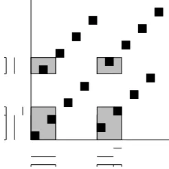
permutation matrix corresponding to a rule’s

per-mutationπ. Figure 1 shows the permutation matrix of rule (2) with a three-step parsing strategy. Each panel shows one combination step along with the projections of the partial results in each dimension; the endpoints of these projections correspond to free boundary variables. The second step has the high-est number of distinct endpoints, five in the vertical dimension and three horizontally, meaning parsing can be done in timeO(N8).

As an example of the impact that the choice of parsing strategy can make, Figure 2 shows a per-mutation for which a clever ordering of partial re-sults enables parsing in timeO(N10_{)in the length} of the input strings. Permutations having this pattern of diagonal stripes can be parsed using this strat-egy in time O(N10_{) regardless of the length n of} the SCFG rule, whereas a na¨ıve strategy proceeding from left to right in either input string would take timeO(Nn+3_).

2.1 Markov Random Fields for Cells

{A, B, C, D}

{A, B, C}

{A, B}

{A} {B} {C}

{D}

x0 x1 x2 x3 x4

y0

y1

y2

y3

y4

A B

C D

x0 x1 x2x3 x4

y0

y1

y2

y3

y4

A B

C D

x0 x1 x2 x3 x4

y0

y1

y2

y3

y4

A B

C D

Figure 1: The tree on the left defines a three-step parsing strategy for rule (2). In each step, the two subsets of nonterminals in the inner marked spans are combined into a new chart item with the outer spans. The intersection of the outer spans, shaded, has now been processed. Tic marks indicate distinct endpoints of the spans being combined, corresponding to the free boundary variables.

(MRF) representation, which will later allow us to use algorithms and complexity results based on the graphical structure of MRFs. A Markov Random Field is defined as a probability distribution2 over a set of variablesx_{that can be written as a product of}

factorsfithat are functions of various subsetsxi of

x_{. The probability of an SCFG rule instance}

com-puted by Algorithm 1 can be written in this func-tional form:

δR(x_{) =P(R)}Y

i

fi(xi)

where

x_{={xi, yi} for0≤i≤n}

x_{i ={xi−1, xi, yπ(i)−1, yπ(i)}}

and the MRF has one factorfifor each child nonter-minalXi in the grammar ruleR. The factor’s value is the probability of the child nonterminal, which can be expressed as a function of its four boundaries:

fi(xi) = δ(Xi, xi−1, xi, yπ(i)−1, yπ(i))

For reasons that are explained in the following section, we augment our Markov Random Fields with a dummy factor for the completed parent non-terminal’s chart item. Thus there is one dummy fac-tordfor each grammar rule:

d(x0, xn, y0, yn) = 1

expressed as a function of the four outer boundary

variables of the completed rule, but with a constant

2_{In our case unnormalized.}

Figure 2: A parsing strategy maintaining two spans in each dimension isO(N10)for any length permu-tation of this general form.

value of 1 so as not to change the probabilities com-puted.

Thus an SCFG rule withnchild nonterminals al-ways results in a Markov Random Field with2n+ 2 variables andn+ 1factors, with each factor a func-tion of exactly four variables.

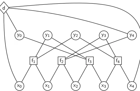
Markov Random Fields are often represented as graphs. A factor graph representation has a node for each variable and factor, with an edge connect-ing each factor to the variables it depends on. An ex-ample for rule (2) is shown in Figure 3, with round nodes for variables, square nodes for factors, and a diamond for the special dummy factor.

2.2 Junction Trees

d

y0 y1 y2 y3 y4

f1 f2 f3 f4

x0 x1 x2 x3 x4

Figure 3: Markov Random Field for rule (2).

message-passing algorithm for graphical models over this tree structure. The complexity of the mes-sage passing algorithm depends on the structure of the junction tree, which in turn depends on the graph structure of the original MRF.

A junction tree can be constructed from a Markov Random Field by the following three steps:

• Connect all variable nodes that share a factor, and remove factor nodes. This results in the graphs shown in Figure 4.

• Choose a triangulation of the resulting graph, by adding chords to any cycle of length greater than three.

• Decompose the triangulated graph into a tree of cliques.

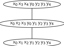
We call nodes in the resulting tree, corresponding to cliques in the triangulated graph, clusters. Each cluster has a potential function, which is a function of the variables in the cluster. For each factor in the original MRF, the junction tree will have at least one cluster containing all of the variables on which the factor is defined. Each factor is associated with one such cluster, and the cluster’s potential function is set to be the product of its factors, for all combina-tions of variable values. Triangulation ensures that the resulting tree satisfies the junction tree property, which states that for any two clusters containing the same variablex, all nodes on the path connecting the clusters also containx. A junction tree derived from the MRF of Figure 3 is shown in Figure 5.

The message-passing algorithm for graphical models can be applied to the junction tree. The

algo-y0 y1 y2 y3 y4

x0 x1 x2 x3 x4

y0 y1 y2 y3 y4

x0 x1 x2 x3 x4

Figure 4: The graphs resulting from connecting all interacting variables for the identity permutation (1,2,3,4)(top) and the (2,4,1,3) permutation of rule (2) (bottom).

rithm works from the leaves of the tree inward, alter-nately multiplying in potential functions and maxi-mizing over variables that are no longer needed, ef-fectively distributing themaxand product operators so as to minimize the interaction between variables. The complexity of the message-passing isO(nNk_), where the junction tree contain O(n) clusters, kis the maximum cluster size, and each variable in the cluster can takeN values.

However, the standard algorithm assumes that the factor functions are predefined as part of the input. In our case, however, the factor functions themselves depend on message-passing calculations from other grammar rules:

fi(xi) =δ(Xi, xi−1, xi, yπ(i)−1, yπ(i))

= max

R′_:Xi→α,β

P(R′) max

x′: x′

0=xi₋₁,x′ n′=xi y′

0=yπ(i₋1),yn′′=yπ(i)

δR′(x′_{) (3)}

We must modify the standard algorithm in order to interleave computation among the junction trees corresponding to the various rules in the grammar, using the bottom-up ordering of computation from Algorithm 1. Where, in the standard algorithm, each message contains a complete table for all assign-ments to its variables, we break these into a sepa-rate message for each individual assignment of vari-ables. The overall complexity is unchanged, because each assignment to all variables in each cluster is still considered only once.

x0x3x4y0y2y3y4

x0x2x3y0y1y2y3y4

x0x1x2y1y2y3y4

Figure 5: Junction tree for rule (2).

tree we derive from an SCFG rule has a cluster con-taining all four outer boundary variables, allowing efficient lookup of the inner maximization in (3). Because the outer boundary variables need not ap-pear throughout the junction tree, this technique al-lows reuse of some partial results across different outer boundaries. As an example, consider message passing on the junction tree of shown in Figure 5, which corresponds to the parsing strategy of Fig-ure 1. Only the final step involves all four bound-aries of the complete cell, but the most complex step is the second, with a total of eight boundaries. This efficient reuse would not be achieved by applying the junction tree technique directly to the maximiza-tion operator in Algorithm 1, because we would be fixing the outer boundaries and computing the junc-tion tree only over the inner boundaries.

3 Treewidth and Tabular Parsing

The complexity of the message passing algorithm over an MRF’s junction tree is determined by the

treewidth of the MRF. In this section we show that,

because parsing strategies are in direct correspon-dence with valid junction trees, we can use treewidth to analyze the complexity of a grammar rule.

We define a tabular parsing strategy as any dy-namic programming algorithm that stores partial re-sults corresponding to subsets of a rule’s child non-terminals. Such a strategy can be represented as a recursive partition of child nonterminals, as shown in Figure 1(left). We show below that a recursive partition of children having maximum complexityk

at any step can be converted into a junction tree hav-ingkas the maximum cluster size. This implies that finding the optimal junction tree will give a parsing strategy at least as good as the strategy of the opti-mal recursive partition.

A recursive partition of child nonterminals can be

converted into a junction tree as follows:

• For each leaf of the recursive partition, which represents a single child nonterminal i, cre-ate a leaf in the junction tree with the cluster (xi−1, xi, yπ(i)−1, yπ(i))and the potential func-tionfi(xi−1, xi, yπ(i)−1, yπ(i)).

• For each internal node in the recursive parti-tion, create a corresponding node in the junc-tion tree.

• Add each variablexito all nodes in the junction tree on the path from the node for child nonter-minali−1to the node for child nonterminali. Similarly, add each variableyπ(i) to all nodes in the junction tree on the path from the node for child nonterminalπ(i)−1to the node for child nonterminalπ(i).

Because each variable appears as an argument of only two factors, the junction tree nodes in which it is present form a linear path from one leaf of the tree to another. Since each variable is associated only with nodes on one path through the tree, the result-ing tree will satisfy the junction tree property. The tree structure of the original recursive partition im-plies that the variable rises from two leaf nodes to the lowest common ancestor of both leaves, and is not contained in any higher nodes. Thus each node in the junction tree contains variables correspond-ing to the set of endpoints of the spans defined by the two subsets corresponding to its two children. The number of variables at each node in the junction tree is identical to the number of free endpoints at the corresponding combination in the recursive par-tition.

Because each recursive partition corresponds to a junction tree with the same complexity, finding the best recursive partition reduces to finding the junc-tion tree with the best complexity, i.e., the smallest maximum cluster size.

Finding the junction tree with the smallest clus-ter size is equivalent to finding the input graph’s

bounded with treewidth results for worst-case rules, without explicitly identifying the worst-case permu-tations.

4 Treewidth Grows Linearly

In this section, we show that the treewidth of the graphs corresponding to worst-case permutations growths linearly with the permutation’s length. Our strategy is as follows:

1. Define a 3-regular graph for an input permu-tation consisting of a subset of edges from the original graph.

2. Show that the edge-expansion of the 3-regular graph grows linearly for randomly chosen per-mutations.

3. Use edge-expansion to bound the spectral gap.

4. Use spectral gap to bound treewidth.

For the first step, we defineH = (V, E)as a ran-dom 3-regular graph on2nvertices obtained as fol-lows. Let G1 = (V1, E1) and G2 = (V2, E2) be cycles, each on a separate set of nvertices. These two cycles correspond to the edges (xi, xi+1) and (yi, yi+1) in the graphs of the type shown in Fig-ure 4. Let M be a random perfect matching be-tweenV1andV2. The matching represents the edges (xi, yπ(i)) produced from the input permutation π. Let H be the union of G1, G2, and M. While H contains only some of the edges in the graphs de-fined in the previous section, removing edges cannot increase the treewidth.

For the second step of the proof, we use a proba-bilistic argument detailed in the next subsection.

For the third step, we will use the following con-nection between the edge-expansion and the eigen-value gap (Alon and Milman, 1985; Tanner, 1984).

Lemma 4.1 LetGbe ak-regular graph. Letλ2 be

the second largest eigenvalue ofG. Leth(G)be the edge-expansion ofG. Then

k−λ2≥

h(G)2 2k .

Finally, for the fourth step, we use a relation be-tween the eigenvalue gap and treewidth for regu-lar graphs shown by Chandran and Subramanian (2003).

Lemma 4.2 LetGbe ak-regular graph. Letn be the number of vertices ofG. Let λ2 be the second

largest eigenvalue ofG. Then

tw(G)≥jn

4k(k−λ2)

k

−1

Note that in our setting k = 3. In order to use Lemma 4.2 we will need to give a lower bound on the eigenvalue gapk−λ2ofG.

4.1 Edge Expansion

The edge-expansion of a set of verticesT is the ra-tio of the number of edges connecting vertices inT

to the rest of the graph, divided by the number of vertices inT,

|E(T, V −T)| |T|

where we assume that|T| ≤ |V|/2. The edge ex-pansion of a graph is the minimum edge exex-pansion of any subset of vertices:

h(G) = min

T⊆V

|E(T, V −T)| min{|T|,|V −T|}.

Intuitively, if all subsets of vertices are highly con-nected to the remainder of the graph, there is no way to decompose the graph into minimally interacting subgraphs, and thus no way to decompose the dy-namic programming problem of parsing into smaller pieces.

Let n_kbe the standard binomial coefficient, and forα∈R, let

n ≤α

=

⌊α⌋

X

k=0

n k

.

We will use the following standard inequality valid for0≤α≤n:

n ≤α

≤ne α

α

(4)

Lemma 4.3 With probability at least0.98the graph Hhas edge-expansion at least1/50.

Proof :

Letε = 1/50. Assume that T ⊆ V is a set with a small edge-expansion, i. e.,

and |T| ≤ |V|/2 = n. Let Ti = T ∩Vi and let

ti = |Ti|, for i = 1,2. We will w.l.o.g. assume

t1 ≤t2. We will denote asℓithe number of spans of consecutive vertices fromEi contained inT. Thus

2ℓi = |E(Ti, Vi −Ti)|, for i = 1,2. The spans counted byℓ1andℓ2correspond to continuous spans counted in computing the complexity of a chart pars-ing operation. However, unlike in the diagrams in the earlier part of this paper, in our graph theoretic argument there is no requirement that T select only corresponding pairs of vertices fromV1 andV2.

There are at least2(ℓ1+ℓ2)+t2−t1edges between

T andV −T. This is because there are2ℓi edges within Vi at the left and right boundaries of the ℓi spans, and at leastt2−t1edges connecting the extra vertices fromT2that have no matching vertex inT1. Thus from assumption (5) we have

t2−t1 ≤ε(t1+t2)

which in turn implies

t1 ≤t2 ≤ 1 +ε

1−εt1. (6)

Similarly, using (6), we have

ℓ1+ℓ2≤ ε

2(t1+t2)≤ ε

1−εt1. (7)

That is, for T to have small edge expansion, the vertices in T1 and T2 must be collected into a small number of spansℓ1 andℓ2. This limit on the number of spans allows us to limit the number of ways of choosing T1 and T2. Suppose that t1 is given. Any pair T1, T2 is determined by the edges in E(T1, V1 −T1), and E(T2, V2 −T2), and two bits (corresponding to the possible “swaps” of Ti with Vi − Ti). Note that we can choose at most

2ℓ1+ 2ℓ2 ≤t1·2ε/(1−ε)edges in total. Thus the number of choices ofT1andT2is bounded above by

4·

2n ≤ ₁2₋ε_εt1

. (8)

For a given choice of T1 and T2, for T to have small edge expansion, there must also not be too many edges that connectT1 to vertices inV2−T2. Let kbe the number of edges between T1 andT2. There are at leastt1+t2−2kedges betweenT and

V −T and from assumption (5) we have

t1+t2−2k≤ε(t1+t2)

Thus

k≥(1−ε)t1+t2

2 ≥(1−ε)t1. (9)

The probability that there are≥(1−ε)t1edges be-tweenT1andT2is bounded by

t1

≤εt1

t2

n

(1−ε)t1

where the first term selects vertices inT1 connected toT2, and the second term upper bounds the proba-bility that the selected vertices are indeed connected to T2. Using 6, we obtain a bound in terms of t1 alone:

t1

≤εt1

1 +ε 1−ε·

t1

n

(1−ε)t1

, (10)

Combining the number of ways of choosing T1 andT2(8) with the bound on the probability that the edgesMfrom the input permutation connect almost all the vertices inT1 to vertices from T2 (10), and using the union bound over values of t1, we obtain that the probabilitypthat there exists T ⊆ V with edge-expansion less thanεis bounded by:

2

⌊n/2⌋

X

t1=0 4·

2n ≤ ₁2₋ε_εt1

t1

≤εt1

1 +ε 1−ε·

t1

n

(1−ε)t1

(11) where the factor of2is due to the assumptiont1 ≤

t2.

to⌊n/2⌋. Using (4) we obtain

p≤8

⌊n/2⌋

X

t1=⌈1₂−εε⌉



 2ne 2ε 1−εt1

!₁2ε −εt1

t1e

εt1 εt1

1 +ε 1−ε·

t1

n

(1−ε)t1# =

8

⌊n/2⌋

X

t1=⌈1₂−εε⌉

e(1−ε) ε

₁2ε −ε e

ε

ε

1 +ε 1−ε

1−ε

t1

n

1−ε− 2ε

1−ε

!t1

.

(12)

We will use t1/n ≤ 1/2 and plugε = 1/50 into (12). We obtain

p≤8

∞

X

t1=25

0.74t1 _≤0.02.

While this constant bound on p is sufficient for our main complexity result, it can further be shown thatpapproaches zero asnincreases, from the fact that the geometric sum in (12) converges, and each term for fixedt1goes to zero asngrows.

This completes the second step of the proof as outlined at the beginning of this section. The con-stant bound on the edge expansion implies a concon-stant bound on the eigenvalue gap (Lemma 4.1), which in turn implies an Ω(n) bound on treewidth (Lemma 4.2), yielding:

Theorem 4.4 Tabular parsing strategies for

Syn-chronous Context-Free Grammars containing rules with all permutations of length n require time

Ω(Ncn)in the input string length N for some con-stantc.

We have shown our result without explicitly con-structing a difficult permutation, but we close with one example. The zero-based permutations of length

p, where p is prime, π(i) = i−1 mod p for0 < i < p, and π(0) = 0, provide a known family of expander graphs (see Hoory et al. (2006)).

5 Conclusion

We have shown in the exponent in the complex-ity of polynomial-time parsing algorithms for syn-chronous context-free grammars grows linearly with the length of the grammar rules. While it is very expensive computationally to test whether a speci-fied permutation has a parsing algorithm of a certain complexity, it turns out that randomly chosen per-mutations are difficult with high probability.

Acknowledgments This work was supported by NSF grants 0546554, 0428020, and IIS-0325646.

References

Albert V. Aho and Jeffery D. Ullman. 1972. The

The-ory of Parsing, Translation, and Compiling, volume 1.

Prentice-Hall, Englewood Cliffs, NJ.

N. Alon and V.D. Milman. 1985. λ₁, isoperimetric inequalities for graphs and superconcentrators. J. of

Combinatorial Theory, Ser. B, 38:73–88.

Stefen Arnborg, Derek G. Corneil, and Andrzej Proskurowski. 1987. Complexity of finding embed-dings in ak-tree. SIAM Journal of Algebraic and

Dis-crete Methods, 8:277–284, April.

L.S. Chandran and C.R. Subramanian. 2003. A spectral lower bound for the treewidth of a graph and its conse-quences. Information Processing Letters, 87:195–200.

Shlomo Hoory, Nathan Linial, and Avi Wigderson. 2006. Expander graphs and their applications. Bull. Amer.

Math. Soc., 43:439–561.

Finn V. Jensen, Steffen L. Lauritzen, and Kristian G. Ole-sen. 1990. Bayesian updating in causal probabilis-tic networks by local computations. Computational

Statistics Quarterly, 4:269–282.

Giorgio Satta and Enoch Peserico. 2005. Some com-putational complexity results for synchronous context-free grammars. In Proceedings of HLT/EMNLP, pages 803–810, Vancouver, Canada, October.

G. Shafer and P. Shenoy. 1990. Probability propaga-tion. Annals of Mathematics and Artificial Intelli-gence, 2:327–353.

R.M. Tanner. 1984. Explicit construction of concentra-tors from generalized n-gons. J. Algebraic Discrete