Modelling diffuse groundwater
recharge in Irish karst
PHILIP SCHULER
A thesis submitted for the degree of Doctor of Philosophy to the
University of Dublin, Trinity College
2020
Department of Civil, Structural and Environmental Engineering
University of Dublin
I declare that this thesis has not been submitted as an exercise for a degree at this or any other university and it is entirely my own work.
I agree to deposit this thesis in the University’s open access institutional repository or allow the Li-brary to do so on my behalf, subject to Irish Copyright Legislation and Trinity College LiLi-brary condi-tions of use and acknowledgement.
Karst aquifers are highly heterogeneous, usually described by a ‘duality of recharge and flow’ or
triple porosities and associated ranges of recharge and flow dynamics comprising laminar (diffuse) and partly or fully turbulent groundwater flow. Such heterogeneity challenges the management re-lated to karst aquifers, including landuse management mitigating contaminant input and transfer (i.e. source protection, etc.), or understanding and mitigating groundwater flooding. Hence, the de-velopment of numerical models for karst aquifers is crucial with regard to improving the under-standing of flow and transport dynamics, as well as providing decision support systems that can incorporate climate change scenarios.
The aim of this research, carried out between 2015 and 2019, is to characterise diffuse recharge and flow components of three distinct autogenic karst aquifers (1. Ballindine spring, a low lying catchment in interaction with a river; 2. Bell Harbour, a coastal-upland catchment impacted by the tide and discharging as submarine and intertidal groundwater discharge; and 3. Manorhamilton spring, an upland-lowland catchment) as basis and part of the development of semi-distributed hy-draulic pipe network models using the urban drainage software InfoWorks ICM. The research ques-tion and objectives comprised: 1.) developing an hydrogeological understanding and conceptual site model (CSM) of each study site; 2.) applying a suitable set of statistical and hydrochemical (time series) analyses to distinguish between recharge and flow components; and 3.) numerically simulate these recharge and flow components in pipe network models, and by doing so, evaluate 1.) and 2.).
Several extensive hydrogeological field investigations had to be carried out in order to improve the conceptual understanding of each catchment as well as to delineate the groundwater catch-ment areas, including continuously automated monitoring of hydroclimatic parameters as well as
‘spot’ field investigations.
Three different types of artificial tracer testswere applied: 1.) ‘classical’ artificial tracer tests using
fluorescent dyes carried out between terrestrial injection sites (e.g. swallow holes) and spring out-lets; 2.) single borehole dilution tests (SBDTs) using the conservative tracer 𝑁𝑎𝐶𝑙 and deionized water; and 3.) tracing submarine groundwater discharge (SGD) using fluorescent dyes injected into terrestrial sites while monitoring is carried onboard of a vessel using a field fluorometer submerged
in the sea sampling ‘mobile’ in transects.
was based on – and carried out hand in hand with - Conceptual Site models (CSM) for each study site: groundwater flow in the Bell Harbour catchment is very complex, integrating deep and shallow flow discharging into the sea with a clear seasonal pattern of ‘low-flow’ vs. ‘high-flow’. The
catchment of Ballindine spring was delineated along the River Robe, which is believed to be a losing stream impacting on the aquifer. Manorhamilton springis a ‘contact type’ spring, largely
controlled by the regional structural pattern, the dip of the formations and the topography.
A combination of time series analysis, including uni- and bivariate statistical methods, fre-quency, noise and multi-resolution analysis (discrete and continuous wavelet transform, cross wavelet transform, wavelet coherence) was applied to support the development of CSMs, but mainly to characterise and quantify different flow components: a concentrated, an intermediate and a low-flow component (LFC). The innovative approach of combining frequency analysis (i.e. Fourier transform) with noise analysis lead to the interpretation of different recharge and flow components towards 3 generic components. The LFC was conceptualised as the component that sustains the lowest discharge of a spring as part of an overall diffuse recharge and flow signal established by using digital recursive filter.
The identified recharge and flow components were incorporated into the developed CSMs and fi-nally numerically simulated in the pipe network models. The 3 different recharge and flow compo-nents were numerically represented in InfoWorks ICM using the soil store and groundwater store of the Ground Infiltration Module (GIM), a rainfall-runoff routing method as well as different discrete flows through pipes, using permeable pipes to simulate Darcian flow and open pipes to model both pressurised and open channel turbulent flows using the Saint-Venant equations to allow the model-ling of time transient effects.
v
I wish to express my sincerest thanks to Laurence Gill for giving me the opportunity to develop this piece of research under his supervision. The confidence I felt was enlightening and motivating, not only for writing paragraphs and running model simulations, but also for the countless times spent in the field to installing, collecting and fixing samplers, rowing out into Bell Harbour Bay, sneaking into turloughs, abseiling into Poll Gonzo and camping on Turlough Hill.
Within the past three to four years, Léa Duran and Paul Johnston were very important sources of knowledge and experience. To both I am very grateful.
In 2009, a four-days field trip along the Vienna Aqueducts led by Christian Maslo opened my eyes for karst and groundwater. Since then, Armin Margane, Ramon Brentführer, Thomas Himmels-berger, Charlotte Wilczok and Jean Abi-Rizk thankfully shared - amongst other things - their ra-tional and profound way of thinking when it comes to karst hydrogeology, research and work-life.
During the period of carrying out this research, many people have directly and indirectly supported me, namely Maurice Brodbeck, Colin Bunce, Kirsty Callaghan, Èlia Cantoni, Mary Curley, David Drew, Natalie Duncan, Eoin Dunne, John Gallagher, Moritz Helmes, Mark Gilligan, Michael Grimes, David Mc Aulay, Ted McCormack, Gerard Mc Granaghan, Malte Janßen, Coran Kelly, Hilde Koch, Denis Korflür, Paul Königer, Monica Lee, Anthony Mannix, Bruce Misstear, Dave Mor-gan, Patrick Morrissey, Kevin Ryan, Fabi Schloz, Pierre-André Schnegg, Leonard Stöckl, Katie Tedd, Patrick Veale, John Walsh, Daniel Wearen.
One major key I have been using to decipher various codes in my life is firstly the ‘education’ I re-ceived from my older siblings Gusche and Toni, and secondly the trust to follow my instincts - which both of my parents Angie and Uli conveyed to me in their own way.
ACF autocorrelation function
BFI baseflow index
BGR Bundesanstalt für Geowissenschaften und Rohstoffe (Federal Institute for Geoscience and Natural Resources)
BOEC Burren Outdoor and Education Centre CSO combined sewer overflow
CSM conceptual site model
CWT continuous wavelet transforms
Co. County
XWT cross wavelet transforms CCF cross-correlation function
𝐴 cross-sectional area
db Daubechies (wavelet)
d day
D detail
2H deuterium
Ø diameter
DEM digital elevation model
𝑄 discharge
DCN Discrete Conduit Network DWT discrete wavelet transforms DOC dissolved organic carbon DOM dissolved organic matter EC electrical conductivity EMMA end member mixing analysis EPA Environmental Protection Agency ET evapotranspiration
FFT fast Fourier Transform
𝑓 friction factor
GSI Geological Survey Ireland GMWL Global Meteoric Water Line GPS global positioning system GIM Ground Infiltration Module GWR groundwater recharge 𝑄𝐺𝑖 groundwater store inflow
GWS Group Water Scheme
Hz hertz
h hour
𝐾 hydraulic conductivity
IS injection site
ICM Integrated Catchment Modelling IAEA International Atomic Energy Agency ITM Irish Transverse Mercator
Jan January (all months abbreviated using the first 3 letters) KGE Kling-Gupta efficiency
l litre
LFC low-flow component
masl m above sea level mbsl m below sea level MI Marine Institute
MRA multi-resolution analysis
nm nanometre
NSE Nash-Sutcliffe efficiency OS observation site
18O oxygen-18
ppb parts per billion P rainfall (precipitation)
𝑎 recession coefficient
𝑘 recession constant
RH relative humidity RMSE root mean square error
R runoff
s second
SRTM Shuttle Radar Topography Mission SBDT single borehole dilution test
S smooth (or residual)
SCS Soil Conservation Service 𝑄𝑟𝑖 soil store inflow
𝛽 spectral exponent
SWMM Storm Water Management Model
SC sub-catchment
SiGD submarine and intertidal groundwater discharge SGD submarine groundwater discharge
T temperature
𝑇𝑐 time of concentration
𝑇𝑝 time of peak flow
TDS total dissolved solids TON Total organic nitrate 𝑇𝑏 total runoff time
TBC tracer break-through curve TCD Trinity College Dublin
TCMA two component mixing analysis
UK United Kingdom
USGS United States Geological Survey VSMOW Vienna Standard Mean Ocean Water VCC volume conservation criteria
Summary ... i
Acknowledgements ... v
Abbreviations ... vii
Table of Contents ... xi
1.
General Introduction ... 1
1.1. Overview ... 1
1.2. Aims and objectives ... 2
1.3. Thesis layout ... 4
2.
State of the Art Review ... 7
2.1. Overview of karst systems ... 7
2.2. Hydrogeology of karst systems ... 12
2.2.1. Groundwater ... 12
2.2.2. Groundwater recharge ... 13
2.2.3. Groundwater flow ... 17
2.2.4. Groundwater discharge ... 21
2.2.5. Baseflow ... 22
2.2.6. Submarine and intertidal groundwater discharge (SiGD) ... 24
2.2.7. Quantifying groundwater flow dynamics in a well or borehole ... 26
2.3. Numerical characterisation of groundwater dynamics ... 27
2.3.1. Time series analysis ... 27
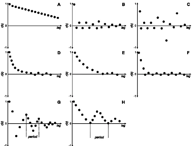
2.3.2. Autocorrelation ... 29
2.3.3. Cross-correlation ... 31
2.3.4. Spectral analysis ... 32
2.3.5. Wavelet analysis ... 38
2.4. Chemical characterisation of groundwater dynamics ... 41
2.4.1. Environmental tracers ... 41
2.4.1.1. Geochemical source tracers ... 42
2.4.1.2. Isotopic tracer ... 42
2.4.2. Artificial tracer hydrology ... 45
2.5. Hydrograph analysis and low-flow separation ... 47
2.5.1. Spring hydrography ... 49
2.5.2. Well/borehole hydrography ... 52
2.5.3. Digital/recursive filtering ... 54
2.5.4. Two-component and end-member mixing analysis ... 57
2.6. Groundwater flow modelling ... 60
2.7 Conceptual elements of an Irish karst aquifer ... 69
3.
Study Sites ... 71
3.1. Ballindine ... 71
3.1.1. Study area ... 71
3.1.2. Geology and structure ... 74
3.1.3. Hydrogeology ... 75
3.2. Manorhamilton ... 77
3.2.1. Study area ... 77
3.2.2. Geology and structure ... 80
3.2.3. Hydrogeology ... 82
3.3. Bell Harbour ... 83
3.3.1. Study area ... 83
3.3.2. Geology and structure ... 86
3.3.3. Hydrogeology ... 88
4.
Materials and Methods ... 93
4.1. Monitoring, sampling and lab analysis... 93
4.1.1. Instrumentation ... 94
4.1.1.1. Field instrumentation ... 94
4.1.1.2. Lab instrumentation ... 101
4.1.2. Meteorological data and processing ... 104
4.1.3. Groundwater and surface water data ... 106
4.1.3.1. Ballindine ... 106
4.1.3.2. Manorhamilton ... 106
4.1.3.3. Bell Harbour ... 106
4.1.4. Tracer techniques ... 110
4.1.4.1. Environmental tracers ... 110
4.1.4.2. Artificial tracers ... 110
4.1.5. Single borehole dilution tests (SBDT) ... 118
4.2. Spatial data sets ... 119
4.3. Methods overview ... 120
4.3.1. Time series analysis ... 120
4.3.1.1. Autocorrelation function ... 121
4.3.1.2. Cross-correlation ... 121
4.3.1.3. Frequency analysis (Fourier transforms) ... 121
4.3.1.4. Wavelet analysis ... 123
4.3.2. Hydrograph analysis and low-flow component separation ... 123
4.3.2.3. Digital recursive filtering ... 127
4.3.2.4. Two-component mixing model ... 127
4.3.3. Quantification of SiGD ... 128
4.4. Numerical modelling ... 131
4.4.1. Lumped modelling ... 131
4.4.2. Pipe network modelling ... 133
4.4.2.1. Hydraulic principles of the model ... 133
4.4.2.2. Translation of general concepts of karst aquifers into InfoWorks ... 146
4.4.2.3. Calibration ... 148
5.
Catchment Studies ... 151
5.1. Ballindine ... 151
5.1.1. Master recession curve analysis ... 154
5.1.2. Water balance ... 159
5.1.3. Tracer tests ... 160
5.1.3.1. Tracer test 08 Aug 2018 ... 161
5.1.3.2. Tracer test 30 Jan 2019 ... 164
5.1.3.3. Conclusions ... 166
5.1.4. Reservoir modelling... 167
5.1.5. Final catchment delineation ... 170
5.1.6. Summary from Ballindine catchment studies ... 171
5.2. Manorhamilton ... 172
5.2.1. Master recession curve analysis ... 174
5.2.2. Event-based recession analysis using stable isotopes ... 178
5.2.3. Water balance ... 181
5.2.4. Tracer tests ... 182
5.2.4.1. Tracer test 16 Sep 2017 ... 183
5.2.4.2. Tracer test 12 Sep 2017 ... 187
5.2.4.3. Conclusions ... 194
5.2.5. Reservoir modelling... 195
5.2.6. Final catchment delineation ... 197
5.2.7. Summary from Manorhamilton catchment studies ... 198
5.3. Conclusions ... 199
6.
Time Series Analysis ... 203
6.1. Autocorrelation ... 203
6.1.1. Ballindine ... 203
6.1.2. Manorhamilton ... 205
6.2.1. Ballindine ... 207
6.2.2. Manorhamilton ... 208
6.2.3. Summary from cross-correlation analysis ... 209
6.3. Spectral and noise analysis ... 209
6.3.1. Ballindine ... 211
6.3.2. Manorhamilton ... 220
6.3.3. Summary from spectral and noise analysis ... 227
6.4. DWT ... 230
6.4.1. Ballindine ... 230
6.4.2. Manorhamilton ... 233
6.4.3. Summary from DWT ... 235
6.5. Low-Flow Component (LFC) separation... 236
6.5.1. Ballindine ... 236
6.5.1.1. Exponential fitting ... 236
6.5.1.2. Digital filtering ... 237
6.5.2. Manorhamilton ... 239
6.5.2.1. Exponential fitting ... 239
6.5.2.2. Digital filtering ... 239
6.5.3. Summary from LFC ... 241
6.6. Conclusions ... 241
7.
Groundwater Modelling using InfoWorks ICM ... 245
7.1. Ballindine ... 245
7.1.1. General model outline... 248
7.1.2. Flow components ... 250
7.1.3. Calibration ... 252
7.1.4. Results ... 255
7.1.5. Summary of Ballindine pipe network model ... 261
7.2. Manorhamilton ... 263
7.2.1. General model outline... 265
7.2.2. Flow components ... 267
7.2.3. Calibration ... 268
7.2.4. Results ... 271
7.2.5. Summary of Manorhamilton pipe network model ... 277
7.3. Conclusions ... 279
8.
Bell Harbour ... 283
8.1. Catchment studies ... 283
8.1.3. Water balance ... 296
8.1.4. Single borehole dilution tests ... 298
8.1.5. Tracer study ... 300
8.1.5.1. Localising areas of SGD ... 301
8.1.5.2. Injection sites ... 302
8.1.5.3. Observation sites... 303
8.1.5.4. Monitoring results ... 305
8.1.5.5. Summary of tracer study ... 311
8.1.6. Conceptual model & catchment delineation ... 312
8.2. Time series analysis ... 313
8.2.1. Autocorrelation ... 313
8.2.2. Cross-correlation ... 317
8.2.3. Signal analysis ... 323
8.2.3.1. Poll Gonzo ... 323
8.2.3.2. BH1 ... 325
8.2.4. DWT ... 327
8.2.4.1. Poll Gonzo ... 327
8.2.4.2. BH1 ... 329
8.2.5. Summary from Bell Harbour time series analysis ... 331
8.3. Low-flow component separation ... 332
8.3.1. BH1 ... 332
8.3.1.1. Exponential fitting ... 332
8.3.1.2. Two-component mixing model ... 334
8.3.2. Poll Gonzo (PG) ... 342
8.3.2.1. Benchmark range for optimal k value ... 342
8.3.2.2. Exponential fitting ... 345
8.3.2.3. Digital filtering ... 346
8.3.3. Summary from Bell Harbour LFC ... 347
8.4. Modelling using InfoWorks ICM ... 347
8.4.1. General model outline ... 348
8.4.2. Flow components ... 352
8.4.3. Calibration ... 353
8.4.4. Results ... 356
8.4.5. Summary from Bell Harbour pipe network modelling ... 361
8.5. Conclusions from Bell Harbour ... 363
9.
Conclusions... 367
1. General Introduction
1.1. Overview
Karstified carbonate aquifers –or ‘karst aquifers’ - exist on all continents in the world, their dis-charge constitutes the largest springs. Moreover, an estimated 25% of the global population re-ceives drinking water that originates from karstified carbonate aquifers (Ford and Williams, 2007). Approx. 22% of the European land surface is characterised by the presence of carbonate rocks (Chen, et al., 2017) presumably karstified to a large extent with such carbonate groundwater re-sources providing an important contribution to the European population’s drinking water supply. For
example, the capital of Austria, Vienna, is almost exclusively supplied by carbonate spring water via a 330 km long-distance carrier (Rihas, 2010). In Ireland, Carboniferous limestone aquifers pro-vide the majority of groundwater supplies (Drew, 2018).
Karstified carbonate aquifers are highly heterogeneous geological formations which are character-ised by multi-scale temporal and spatial hydrological behaviour. Karst aquifers are usually de-scribed in terms of two or three distinct types of porosity models: matrix, fracture and conduit per-meabilities (White and White, 2005). Multiple perper-meabilities relate to different fluid flow dynamics within such systems. This is usually summarised as fast conduit flow vs. slow matrix/fracture flow,
described by the “duality of karst aquifers” in relation to infiltration, flow and discharge (Kiraly, et al., 1995). Accordingly, the availability of quantitative information about these different flow processes is crucial as it is ultimately linked to the appropriate management and protection of karst groundwa-ter.
A major challenge in the quantitative analysis of karst aquifers is the combined dynamics of these different permeabilities, which build up the architecture of properties of such an aquifer. The intrin-sic properties of an aquifer constitute a unique signature that drives infiltration, flow and discharge over space and time. Information about these processes and aquifer properties can be studied us-ing time-amplitude signals, e.g. a karst sprus-ing hydrograph, which describes the hydrodynamic re-sponse observed at the spring outlet to an input signal (e.g. rainfall). A given discharge rere-sponse measured at a spring characterises the rainfall signature as well as the global structure of the drained aquifer. Following a rain event, each hydrograph shows a unique recession response. Such recession describes exponential courses following the principles of emptying nonlinear reser-voirs (Chang, et al., 2015) or much more commonly applied linear reserreser-voirs (Maillet, 1905). Ac-cordingly, the different components of permeability making up a karst aquifer can be conceptual-ised as distinct reservoirs.
series of exponential curves onto the entire recession of a karst hydrograph resembling the differ-ent permeabilities in the karst aquifer (Forkasiewicz and Paloc, 1967). Today, the separation of karst spring recession into a slow-flow baseflow component and fast flowing flood components is widely accepted.
Different methods for separation or decomposition of the baseflow component from the total hydro-graph or only recession are available ranging between numerical approaches such as digital recur-sive filtering (Chapman, 1999) and numerical baseflow separation (Kovács, et al., 2005; Kovács and Perrochet, 2008; Kovács, et al., 2015) or chemical approaches such as two component mixing analysis (TCMA) or end-member mixing analysis (EMMA) using for example stable isotopes (18O, 2H) (Fritz, et al., 1976; Laudon and Slaymaker, 1997). Further, signal analysis in the form of
multi-resolution analysis (MRA) (Torrence and Compo, 1998; Labat, et al., 2000b) may evolve as a po-tential method for baseflow separation.
Complementary to the approaches of baseflow separation, numerical groundwater modelling can be applied in order to infer information about - and simulate - different groundwater flow dynamics, including the slow-flow component. Different modelling approaches exist ranging between global (lumped) and fully distributed approaches. The models and/or the interpretation of their results are all challenged by the heterogeneity of karst aquifers.
In the Irish context, semi-distributed pipe network models have been proven to excel well in the context of karst aquifers with a high proportion of fast-flow components in the conduit permeability domain. Yet, until now, the fissured matrix permeability and its slow-flow components was not suffi-ciently represented in terms of linking such flow components to a measured of quantified contribu-tion.
The purpose of this research is therefore to identify and study the slow-flow dynamics in three Irish karst aquifers (Ballindine, Bell Harbour and Manorhamilton) by means of baseflow separation using a combination of different techniques. A set of different methods is applied to separate the
baseflow component of karst springs, which is considered to be representative for diffusely infiltrat-ing rainfall and slow-flow components originatinfiltrat-ing from the low permeability domain. The resultinfiltrat-ing baseflow time series have then been specifically used as reference for a semi-distributed numerical pipe network modelling approach using InfoWorks ICM alongside the heretofore more resolved fast-flow component originating from the conduit domain.
1.2. Aims and objectives
realistic numerical models of these aquifers. For example, such models can then be used to make predictions as to the aquifer response due to climate change, develop engineering solutions to po-tential flooding predictions or to evaluate contaminant transport and landuse options.
The project objectives are to:
1. Provide a hydrogeological assessment of each catchment: quantify its discharge and rep-resentative rainfall over at least one hydrological year, establish water balances, delineate the catchment boundaries, assess flow dynamics and develop conceptual site models (CSM) as basis for a profound hydrogeological understanding as basis for any recharge-discharge assessments;
2. Differentiate between slow (diffuse) and fast (concentrated) recharge and flow into and within a karst network using both chemical (isotopic and trace element water quality) and numerical and statistical approaches towards spring hydrograph separation, and quantify the flow and response times of diffusely recharged flow;
3. Develop numerical (pipe network) models of the three karst aquifers that allow to distin-guish different flow components as a result of the intrinsic heterogeneity of the aquifer and the CSM.
The numerical modelling approach is based on the principles applied in the lowland karst area of south Galway in the west of Ireland which accurately simulates the temporal flooding dynamics of the turloughs on the network (Gill, et al., 2013a). This modelling approach has worked well with re-spect to the groundwater – surface water interactions (water levels in the ephemeral lakes known as ‘turloughs’) but it is recognised that it is limited as to the accuracy of the representation of the diffuse autogenic recharge into the network. Such autogenic recharge is of significant interest par-ticularly with regard to contaminant transport and attenuation across such catchments.
Hence, this research investigates three different karst networks all with autogenic recharge, but each with different characteristics found in the Irish context: a lowland karst aquifer (Ballindine, County (Co.) Mayo); a upland-lowland karst aquifer (Manorhamilton, Co. Leitrim); and a complex coastal-upland karst aquifer (Bell Harbour, Co. Clare).
This research focusses on characterising diffuse - but also concentrated - recharge and flow through the karst system in these three different aquifers by applying different investigative tech-niques. The investigative techniques involve both chemical (stable isotopes and ions) and statisti-cal and numeristatisti-cal methods, such as hydrograph separation techniques, time series analysis Includ-ing uni- and bivariate methods, Fourier analysis coupled with noise analysis and multi-resolution analysis (MRA).
In addition, numerical analysis of the spring hydrographs of Ballindine and Manorhamilton, which represent the global aquifer response, are used to differentiate the fast aquifer and spring response following rain events as opposed to the slower more diffuse response.
This research trials different numerical techniques such as discrete wavelet techniques and noise analysis (Schroeder, 1991; Beier and Hardy, 1996; Fournillon, 2012) to investigate the inherent non-linear, non-stationery natural hydrological processes in such a karst system.
1.3. Thesis layout
The three study sites differ significantly from each other. Ballindine and Manorhamilton constitute terrestrial inland karst catchments with more or less well-defined discharge locations. In turn, the catchment of Bell Harbour is a coastal terrestrial-marine aquifer that is impacted by the sea and its tide, and it is drained via multiple intertidal and submarine outlets. Within this project, much re-search had to be conducted to understand the system of Bell Harbour to a level that is necessary for recharge-discharge analyses. In fact, the amount of work put into Bell Harbour significantly ex-ceeds respective workload for Ballindine and Manorhamilton.
Further, some different approaches were applied in Bell Harbour as opposed to the other two sites. These circumstances were acknowledged in the structure of this work. Accordingly, at first, results are presented and compared between Ballindine and Manorhamilton. Conclusions from that are then used and applied on the catchment of Bell Harbour, which is presented at last.
The thesis is structured as follows: The conceptual understanding of karst aquifers underlying this
research is summarised within ‘State of the Art Review’. Further, this chapter presents the literature
on different methods related to hydrograph separation, numerical and chemical characterisation of karst aquifers and groundwater flow modelling.
Chapter ‘Study Sites’ introduces the three karst systems, including their delineated catchment boundaries resulting from this research. Chapter ‘Materials and Methods’ presents the primary and secondary data that was used in this study, sampling and lab analysis, as well as the main statisti-cal and numeristatisti-cal methods for hydrograph separation and groundwater modelling, tracer testing, and quantifying of submarine and intertidal groundwater discharge (SiGD) applied in Bell Harbour.
Chapter ‘Catchment Studies’ presents the process of delineating the catchment boundaries of Ball-indine and Manorhamilton using water balances, reservoir modelling and artificial tracer tests. Fur-ther, the average recession, namely the master recession curve (MRC) is used to characterise both aquifers with regard to recharge, flow and discharge. Both systems are then numerically and
flow modelling using InfoWorks ICM® (version 7.0.5., Innovyze Ltd., Wallingford, UK) presented in Chapter ‘Groundwater Modelling using InfoWorks ICM’, finalising the analyses on Ballindine and
Manorhamilton.
Finally, Chapter ‘Bell Harbour’ presents all results achieved for the coastal system of Bell Harbour. In a similar way to the Ballindine and Manorhamilton catchments, the studies that have informed the understanding of the global functioning of the system, as well delineation of the catchment boundaries, are first presented. Bell Harbour has proven to be a complex multi-level coastal karst aquifer, which had to be examined extensively using a high resolution hydrometeorological moni-toring network along with discrete sampling and tracer testing. The synthesis of results was applied on a numerical model, which in turn yields additional information on groundwater flow dynamics.
2. State of the Art Review
2.1. Overview of karst systems
The term ‘karst’ can be tracked back to pre-Indoeuropean origins. In the context of karst hydrogeol-ogy, the more recent origin in Slovenia is of relevance where the word ‘kar(r)a’ underwent the evo-lution via ‘kars’ to ‘kras’, which means stoney, barren ground (Ford and Williams, 2007). Ultimately, karst describes a landscape that is developed on especially soluble rocks such as limestone, mar-ble, and gypsum. In the introduction of their seminal publication, Ford and Williams (2007) highlight the two key aspects of karst landscapes, i.e. a) the groundwater/hydrogeology domain, and b) the karst landscape/geomorphology domain, both above and below the surface. It is important to note, especially for this study, that an absence of features above the ground doesn’t imply an absence of features below the ground.
The existence of karst and karst features is ultimately linked to the geological structure providing the framework for preferential dissolution, and to the underlying lithology and mineralogy that al-lows for the development of karst, i.e. ‘karstification’, caused by the process of chemical solution of rocks. In Ireland, karst features are documented in >80% of the limestone outcrops indicating wide-spread karstification (Drew, et al., 1996). Karstification is related to the presence of ‘karst minerals’
belonging to three classes, i.e. carbonate minerals (e.g. calcite, dolomite), sulphate minerals (gyp-sum, anhydrite), and halide minerals (halite) (Goldscheider and Andreo, 2007). Of most importance and relevance to this study is the group of carbonate minerals, which are composed of the car-bonate anion (𝐶𝑂32−). The most important karst mineral is calcite (𝐶𝑎𝐶𝑂3), which - if predominantly
present - forms limestone, i.e. a carbonate rock. Another relevant karst mineral is dolomite, which forms dolostone or dolomite. Dolomite is an anhydrous carbonate mineral composed of calcium magnesium carbonate (𝐶𝑎𝑀𝑔(𝐶𝑂3)2).
Carbonate rocks are all types of sedimentary or metamorphic rocks with >50% carbonate minerals in weight (Ford and Williams, 2007; Goldscheider and Andreo, 2007). Depending on the percent-age of calcite or dolomite, as well as impurities, carbonate rocks may be classified according to Figure 2.1.
Figure 2.1: Bulk compositional classification of carbonate rocks (Ford and Williams, 2007).
Carbonates are considered to have a ‘primary porosity’ that describes all pore space present im-mediately after final deposition, and a ‘secondary porosity’ and ‘tertiary porosity’ that are created after final deposition (Choquette and Pray, 1970; Teutsch and Sauter, 1991). The effective porosity of carbonates is of major importance as it directly influences the permeability, i.e. hydraulic conduc-tivity, of rocks, hence, enabling flow and storage of groundwater. More precisely, it is the effective porosity, i.e. the interconnected pore space (excluding only localised openings) that must be con-sidered as only this proportion of the overall bulk porosity allows free gravity flow of groundwater (Kresic, 2007). Newly deposited carbonates have a porosity of 40-70%, but this drops to a few per-cent as the rock consolidates over time (Choquette and Pray, 1970).
Many of the important changes in sedimentary carbonates and their pore systems occur near the surface, either very early in burial history or at later stage in relation to erosion and uplift
(Choquette and Pray, 1970). Tectonics and mechanical stress often impact on the rock matrix, which is visible today as subvertical fractures such as joints or veins. Joints may be stratabound with regular spacing forming the characteristic geometrical fracture networks of grykes and clints on the outcrop surface. Joints are relatively shallow and may be limited to limestone mechanical units. In turn, veins, which developed in deeper depths across strata, are therefore non-strata-bound and are scale-independent (Gillespie, et al., 2001).
The dissolution of carbonates differs between rocks. Limestones are generally more karstifiable than dolostone whereas the karstifiability of a rock decreases with increasing impurity caused by clay content, for example. Other impurities that impact on the chemistry of groundwater may be re-lated to mineralisation, including for example sulphate (𝑆𝑂42−) that is derived from the slow
oxida-tion of pyrite (𝐹𝑒𝑆2) (Tooth and Fairchild, 2003).
The dissolution (or karstification) of carbonate rock is described by the process of acid dissolution, a sequence of reactions. Eqn. 2.1 describes the reaction of limestone in water, i.e. the dissociation, which in fact is small for limestone in pure water. However, in presence of a free proton 𝐻+, the
se-quence of reactions Eqn. 2.1 and Eqn. 2.2 become active,
𝐶𝑎𝐶𝑂3⇔ 𝐶𝑎2++ 𝐶𝑂32− Eqn. 2.1
𝐶𝑎2++ 𝐶𝑂
32−+ 𝐻+⇔ 𝐶𝑎2++ 𝐻𝐶𝑂3− Eqn. 2.2
𝐶𝑂32− becomes hydrated to form soluble bicarbonate 𝐻𝐶𝑂3−. The process depends on the saturation
of given minerals in the solution as well as the availability of 𝐶𝑂2 which forms carbonic acid. The
concentration of carbonic acid is affected by different factors, such as microbial activity in the soil which in turn depends on the soil temperature (Tooth and Fairchild, 2003). Yet, more importantly, the rate of limestone dissolution is four orders higher in turbulent flow compared to laminar flow (Dreybrodt, 2004), enabling speleogenesis to progress.
Within the saturated zone, with increasing vertical depth, the saturation of 𝐻𝐶𝑂3− generally
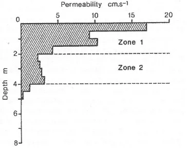
in-creases and the rate of dissolution dein-creases. This phenomenon results in the potential presence of a highly karstified or weathered upper zone of a karst aquifer, i.e. subcutaneous zone, or
[image:33.595.100.282.573.717.2]‘epikarst’ (Mangin, 1975) of high permeability (Figure 2.2) usually diminishing exponentially with depth over typically 3 to 10 meters (Ford and Williams, 2007). However, in Ireland, if present, the epikarst may be limited to a depth of only 1 m (Williams, 2008).
The ‘epikarst’ has been conceptualised as a sub-system of the karst aquifer largely influencing the recharge dynamics of the aquifer (Figure 2.3) (Kiraly, et al., 1995; Bakalowicz, 2004). Below the upper weathered zone or epikarst, a karst aquifer is commonly conceptualised by a hierarchical network of flow paths in the form of a matrix embedded in a network of fissures, fractures and con-duits enlarged by dissolution and flow kinetics (Figure 2.5).
Figure 2.3: Schematic of the epikarst (E) with concentrated (A) and diffuse (B) infiltration (Mangin, 1975; Kiraly, et al., 1995).
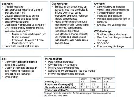
Conduits, fractures and the matrix have distinct properties and functioning within carbonate aqui-fers. In a comprehensive review on carbonate aquifers, Worthington, et al. (2000) conclude that the permeability structure following dissolutionally enlarged networks applies to all unconfined car-bonate aquifers (dolostone, limestone and chalk) irrespectively of the deposition age. The authors provide average hydraulic properties of the three different permeabilities, which previously had more commonly been stated for aquifers or strata as a whole. Generally, the matrix accounts for the largest share of porosity and the highest proportion of groundwater storage with the lowest hy-draulic conductivities and lowest proportion of overall groundwater flow. Conversely, conduits ac-count for the largest proportion of groundwater flow related to the highest hydraulic conductivities, low proportions of storage and very low porosities. The fracture domain is somewhat between the conduit and matrix domain, with a low proportion of groundwater flow, moderate hydraulic conduc-tivities, low proportions of storage and low porosity. For example, Worthington, et al. (2000) provide an average porosity, proportion of storage, hydraulic conductivity and proportion of flow for the three permeabilities for the prominent limestone system of the Mammoth cave area of Mississip-pian age (Table 2.1).
It becomes evident that the matrix and its porous structure has a negligible influence on groundwa-ter flow in the exemplified limestone aquifer (as opposed to chalk). Yet, many (groundwagroundwa-ter flow
modelling) studies related to limestone aquifers refer to a ‘matrix domain’ and groundwater flow
2012), which may cause confusion from a geological point of view. However, all these referred au-thors consider the matrix domain as ‘fissured’ or ‘fractured’ (porous) matrix domain, abbreviated as ‘matrix domain’. Hence, the term ‘matrix’ incorporates some level of secondary porosity, i.e.
(nar-row) fissures/fractures.
Table 2.1: Average hydraulic properties of the matrix, fractures and conduits of the Mammoth Cave limestone aquifer (Worthington, et al., 2000).
Property Matrix Fracture Conduit
Porosity [%] 2.4 0.03 0.06
Proportion of storage [%] 96.4 1.2 2.4
Hydraulic conductivity [m/s] 2 x 10-11 1 x 10⁻⁵ 3 x 10⁻³
Proportion of flow [%] 0.00 0.3 99.7
Mature karst systems include different porosities and permeabilities ranging between the primary porosity of the matrix and larger conduits (Figure 2.4). Most commonly, permeabilities are ex-pressed as a) matrix (µm to mm opening), b) fractures (10 µm to 10 mm) and c) conduits (>10 mm) (Ghasemizadeh, et al., 2012).
Figure 2.4: Types pf porosities in carbonate aquifers with geometrical dimensions, modified after White (1988).
Referring to the abovementioned characteristics, a karst aquifer may be defined according to Hun-toon (1995) as “an aquifer containing soluble rocks with a permeability structure dominated by
in-terconnected conduits dissolved from the host rock which are organized to facilitate the circulation of fluid on the downgradient direction wherein the permeability structure evolved as a consequence
of dissolution by fluid”. Furthermore, to refer to the introduction of this section, a karst aquifer differs
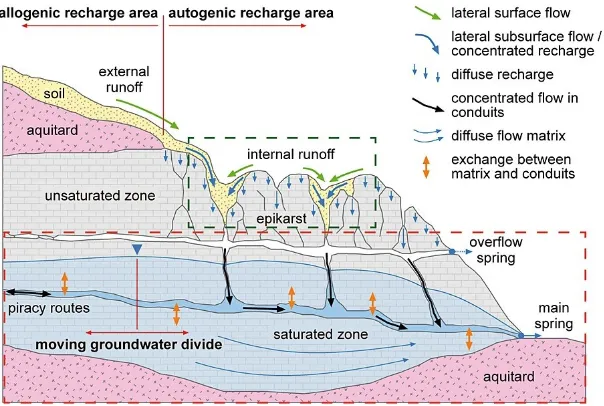
Figure 2.5: Conceptual model of a karst system including diffuse recharge and concentrated re-charge into the conduits (Hartmann, et al., 2014a).
2.2. Hydrogeology of karst systems
2.2.1. Groundwater
Freeze and Cherry (1979) refer to groundwater as subsurface water that occurs beneath the water table in soils and geologic formations that are fully saturated. This definition relates groundwater to the saturated, i.e. phreatic, zone, and it further implies the existence of a water table, whose exist-ence has been subject to controversial discussion in the context of karst aquifers. White (1988) ar-gued that the nature of a water table in karst needs to be considered. This nature is dynamic, and therefore, in certain areas, the water table may just be very irregular, yet present. However, a water table refers to an unconfined aquifer in which water freely moves under gravity forming the piezo-metric surface (Ford and Williams, 2007). There, the pressure head at the water table equals the atmospheric pressure. In turn, within confined systems, the pressure head may exceed the water table. The imaginary surface of interpolated pressure heads is called the ‘potentiometric surface’.
Figure 2.6: Change of the piezometric surface according to the change in the drainage regime be-tween a) baseflow and b) flood conditions (Gunn, 2004).
Within the context of the Water Framework Directive (WFD) of the European Union (EU), ground-water is defined as “all water which is below the surface of the ground in the saturation zone and in
direct contact with the ground or subsoil” (EPA, 2006). This definition does not consider the exist-ence or concept of a water table. In fact, the majority of karstified limestone aquifers in Ireland are
considered as ‘low lying’ cropping out <100 m above sea level (masl) (Drew, 2008). These areas are characterised by a very shallow unsaturated zone and seasonal groundwater flooding via tur-loughs (Naughton, et al., 2012). Turtur-loughs are described as topographic depressions in karst which are intermittently flooded on an annual cycle via groundwater sources and have substrate and/or ecological communities characteristic of wetlands (EPA, 2004).
Turlough water levels constitute a visible potentiometric surface of the aquifer rather than a piezo-metric surface. Therefore, in the context of low lying topography and a shallow unsaturated zone, the notation of a potentiometric surface rather than a piezometric surface or water table is favoura-ble working on the scale of an entire aquifer. Accordingly, the definition of groundwater by EPA (2006) is extended to account for the heterogeneities in karst, where ‘groundwater is all water be-low the surface in the ground in the saturated zone and in direct contact with the ground or subsoil forming a potentiometric surface over the aquifer unit’.
2.2.2. Groundwater recharge
Because of the heterogeneity of karst aquifers constituted by different permeabilities (White, 1988), karst groundwater recharge occurs on different scales. Groundwater recharge may be described as
the “entry into the saturated zone of water made available at the water table surface, together with
Recharge to an aquifer can originate from the karst area itself (autogenic) or from adjacent non-karst areas (allogenic) (Goldscheider, et al., 2007). Further, two types of recharge can be distin-guished, a) direct (vertical infiltration of precipitation where it falls on the ground) and b) indirect (in-filtration following runoff) (Misstear and Brown, 2007).
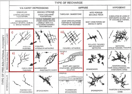
The role of groundwater recharge on the evolution of caves and conduits is displayed in Figure 2.7, distinguishing between concentrated recharge (via depressions), diffuse and hypogenic with spect to different types of psolutional porosity. Of relevance for this study is concentrated re-charge via swallow holes into bedding partings and fractures and diffuse rere-charge through sand-stone into bedding partings and fractures. Even though none of the study sites in this research
pro-ject receive allogenic recharge from sandstone at present (see ‘Study Sites’), allogenic recharge
[image:38.595.61.497.295.605.2]may have been the case in the past explaining the current hierarchy of dissolution pathways.
Figure 2.7: Relationship between geomorphology and groundwater recharge. Modified after Ford and Williams (2007).
Karst aquifers have been largely conceptualised as two component systems, distinguishing be-tween concentrated flow and recharge vs. diffuse flow and recharge (Atkinson, 1977). Concen-trated or direct recharge occurs usually very rapidly and highly localised into the conduit system. In turn, diffuse groundwater recharge occurs over an entire catchment area entering the low permea-bility fissured matrix blocks rather slowly (Geyer, et al., 2008b). In fact, diffuse groundwater
i)
ii)
iii)
recharge follows the hierarchical network of flow paths enlarged by dissolution, as it is shown in Figure 2.7iv, eventually discharging into conduits and drained by springs. Depending on the evolu-tion of the karst system, diffusely recharged groundwater will travel through different sized open-ings, from small fissures towards conduits. Accordingly, diffuse groundwater recharge will experi-ence different flow dynamics, i.e. laminar through to fully turbulent flow. This conceptual under-standing is illustrated as part of the overall functioning of a karst aquifer in Figure 2.5.
Additional complexity is associated with the epikarst and its role in the recharge process. The epikarst may form a perched and shallow - potentially saturated - unit from where water infiltration is concentrated or via diffuse flow paths, depending on the magnitude of recharge, saturation of the epikarst with relatively short residence times and piston-like functioning (Perrin, et al., 2003; Aqui-lina, et al., 2006). The first reference to epikarst in the Irish context was provided by Daly (1997). The presence of an epikarst layer that acts like a reservoir may be subject to debate at a site-spe-cific level as epikarst is not ubiquitous. The epikarst simply may not have formed or it may have been scoured off by glacial processes eroding off the weathered zone. As a result, such weathered zone may be limited to 1 m depth, as exemplified in the Burren, western Ireland (Williams, 2008). Since much of Ireland was impacted by glacial erosion in the past, the vertical depth, and hence the role of the epikarst in recharge processes may be considered as limited.
Further complexity in recharge processes is added by considering the soil layer and its properties, including different flow routes, namely slow matrix flow (a) and rapid macropore flow (b, c) (Figure 2.8). Such different permeabilities are related to the conceptual dual porosity properties of soils, for example in the case of a clay-dominated glacial till (Tooth and Fairchild, 2003), which is very com-mon in Ireland. Rapid flow occurs through cracks and macropores, also called bypass flow (or pref-erential flow paths). For example, bypass flow may occur in periods of soil moisture deficit (Rush-ton and Ward, 1979). In turn, micropores exhibit the large storage capacity, e.g. in till, providing constant delivery of matrix flow. Groundwater recharge originating from slow matrix flow is associ-ated with the baseflow sustaining the low flow, and generally with a slow groundwater flow dynamic (Tooth and Fairchild, 2003).
The quantification of groundwater recharge is very difficult as it is not directly measurable. Indirect methods for quantifying recharge rely on chemical measurements (e.g. tracers) and/or physical measurements (e.g. water content, water table fluctuation) (Ireson and Butler, 2013). The use of water table fluctuations, however, is based on the premise of an existing water table, which may be the case in certain carbonates, such as chalk, but which is considered not necessarily to be the case in karstified limestone. Further, hydrochemical approaches or water budget estimations tend to require lots of site-specific parameters. While there are numerous studies on groundwater re-charge, e.g. in the chalk of the UK, based on the premise of a groundwater table (Mathias, et al., 2006; Van den Daele, et al., 2007; Ireson, et al., 2009), the contrary is the case for limestone aqui-fers in Ireland or indeed other comparable shallow and low lying limestone aquiaqui-fers more interna-tionally on which this research could refer to.
However, importantly, groundwater recharge impacts on the shape and magnitude of groundwater discharge in time. This is perhaps the most fundamental premise for this research, as it allows
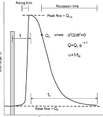
re-charge to be approached from the ‘disre-charge perspective’. With the beginning of effective recharge during an event impacting on the phreatic zone, spring discharge increases – the spring hydro-graph rises. At the time of maximum recharge an inflection point can be identified on the rising limb of the spring hydrograph (Figure 2.9i). Another inflection point occurs at the end of the recharge event on the falling limb (Figure 2.9ii). The falling limb can be sub-divided into different recession components, such as the flood recession and the baseflow recession (Kovács, et al., 2005; Geyer, et al., 2008b). Hence, analysis of the falling hydrograph, i.e. recession analysis, allows conclusions to be drawn with respect of the recharge event (Mangin, 1975). This understanding allows conclu-sions to be drawn on groundwater recharge dynamics from the analysis of spring hydrographs, which again forms the underlying principle of this study.
Figure 2.9: Typical spring hydrograph as response to recharge with inflection points for the time of maximum recharge (i) and for the end of the recharge event (ii). Modified after Kovács, et al. (2005).
Recharge
The relevance of the epikarst influencing recharge volumes of the low permeability domain and consequently impacting the baseflow of spring hydrographs of a heterogeneous aquifer was nu-merically justified by Kiraly, et al. (1995). In fact, the epikarst may be conceptualised as a storage reservoir that drains as a baseflow component, or as a quick-flow component. The characteristic of the drainage may depend on the saturation of the epikarst with relatively short residence times and piston-like functioning (Perrin, et al., 2003; Aquilina, et al., 2006). Accordingly, the epikarst may be interpreted as a perched aquifer, and where present, its drainage may influence the spring hydro-graph and its chemohydro-graph.
2.2.3. Groundwater flow
Groundwater flow is a physical process along a gradient where the potential may be defined as a
“physical quantity, capable of measurement at every point in a flow system, whose properties are such that flow always occurs from regions in which the quantity has higher values to those in which
it has lower, regardless of the direction in space” (Hubbert, 1940). Different potential gradients im-pact on the motion of groundwater, such as a temperature gradient, electrical gradient, chemical gradient and a hydraulic head gradient. The consideration of multiple potentials in the quantification
of groundwater flow is called ‘coupled flow’. However, within the saturated zone of an aquifer, groundwater flow may be fully described by hydraulic head (elevation + pressure components) and hydraulic conductivity (Freeze and Cherry, 1979).
Accordingly, in a porous, isotropic and homogeneous medium, groundwater flow in the saturated
zone can be approximated by linearity and Darcy’s law (Darcy, 1856) where,
𝑢 = −𝐾𝑑ℎ 𝑑𝑙 =
𝑄
𝐴 Eqn. 2.3
with the specific discharge 𝑢, the hydraulic conductivity 𝐾, the hydraulic gradient 𝑑ℎ/𝑑𝑙, discharge 𝑄 and the cross-sectional area of the granular medium 𝐴. Darcy’s law (or rather, empirical study) describes a linear relationship between 𝑢 and 𝑑ℎ/𝑑𝑙 and laminar flow, in which conceptually water molecules move in parallel to the direction of flow. There is an upper and lower limit for the validity of this linear relationship, of which the upper limit is of relevance in karst hydrogeology. At high flow
rates, Darcy’s law is not valid anymore. A threshold that distinguishes between laminar flow and the application of Darcy’s law and non-laminar or turbulent flow at higher velocities is given by the dimensionless Reynolds number 𝑅𝑒. In fact, 𝑅𝑒 describes the state of flow given as,
𝑅𝑒=𝜌𝑢𝑑𝜇 Eqn. 2.4
of the permeability 𝑘. The transition between laminar and turbulent flow is expressed by the critical Reynolds number 𝑁𝑅𝑒 that depends on the hydraulic properties of the fluid and the pore space. For
porous media, the generally accepted range of laminar flow applies to 𝑅𝑒 in the range between 1 to
10 (Zeng and Grigg, 2006) (Figure 2.10). Above 𝑁𝑅𝑒, flow is fully turbulent in porous media (Freeze
and Cherry, 1979; Giese, et al., 2018).
Figure 2.10: Range of validity of Darcy's law (Freeze and Cherry, 1979).
However, karst aquifers cannot be approached by the assumption or simplification of acting like a
‘porous, isotropic and homogeneous medium’. Instead, karst is a medium of preferential flow paths, including conduits, which are similar to pipes. In pipes, laminar flow usually applies to 𝑅𝑒 <2,000
(Mays, 2011) while turbulent flow is considered to start at 𝑁𝑅𝑒 of 500 to 2,000, where 𝑁𝑅𝑒 being
site-specific with regard to each karst system or sub-system (Giese, et al., 2018). The change of flow regimes is transitional.
Laminar flow through pipes, which may be realistic representations of conduits, may be
ap-proached by Poiseuille’s law or with the Hagen-Poiseuille equation as,
𝑄 =𝜋𝑑
4𝜌𝑔
128𝜇 × 𝑑ℎ
𝑑𝑙 Eqn. 2.5
with the gravitational acceleration 𝑔, and the fluid density 𝜌 and viscosity 𝜇 (Ford and Williams, 2007).
𝑄 = (2𝑑𝑔𝑎
2
𝑓 )
1/2
× (𝑑ℎ 𝑑𝑙)
1/2
Eqn. 2.6
with the friction factor 𝑓 (Ford and Williams, 2007) defined according to the Darcy-Weisbach friction law,
𝜏 =𝑓𝜌𝑓
8 × 𝑣2 Eqn. 2.7
with the shear stress 𝜏, the density of fresh water 𝜌𝑓 and the mean velocity through a pipe 𝑣.
Another way to estimate the friction factor 𝑓 is to apply the Colebrook-White equation (Colebrook and White, 1937). Different forms of the Colebrook-White equation exist, e.g.
1
√𝑓= −2 log10 𝜀 3.71𝐷+
2.51 𝑅𝑒√𝑓
Eqn. 2.8
with the absolute roughness coefficient 𝜀 and the inner pipe diameter or hydraulic radius 𝐷
(Rollmann and Spindler, 2015). Hence, the Colebrook-White equation relates the friction factor, the Reynolds number, pipe roughness and the inside pipe diameter. In karst conduits, 𝑓 may range be-tween 0.1 and 340 (Jeannin, 2001).
While the abovementioned flow types through porous medium and fractures/fissures and pipes may be valid for saturated conditions and specific geometries, there often is also unsaturated open-channel flow occurring in karst aquifers. Conduits that drain fractures, fissures and the matrix may be not fully saturated in periods of recessions following recharge events (Figure 2.6). Shallow water flow as occurring in under-pressurized conduits influenced by the atmosphere is generally ap-proached by using the Saint-Venant equations of conservation of mass and momentum unsteady open channel flow (Gill, et al., 2013a),
𝛿𝐴 𝛿𝑡 +
𝛿𝑄
𝛿𝑥 = 0 Eqn. 2.9
𝛿𝑄 𝛿𝑡 +
𝛿 𝛿𝑥(
𝑄2
𝐴) + 𝑔𝐴 (cos 𝜃 𝛿𝑦 𝛿𝑥− 𝑆0+
𝑄|𝑄|
𝐾2 ) = 0 Eqn. 2.10
with the discharge 𝑄 [m3/s], the cross-sectional area 𝐴 [m2], the acceleration due to gravity 𝑔 [m/s2],
the angle of bed to horizontal (º) 𝜃, the bed slope 𝑆0 and the conveyance 𝐾. The conveyance may
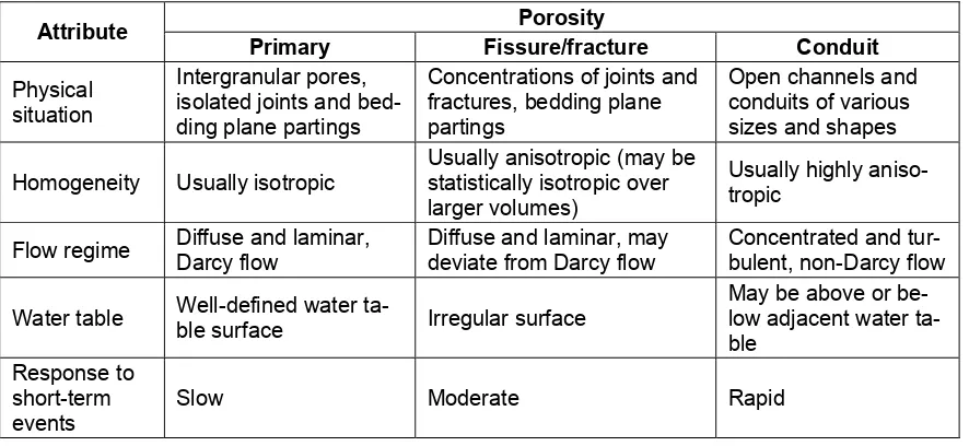
The type of groundwater flow occurring depends on the geometries of openings, which is related to the type of porosity and aquifer characteristics, ranging between laminar flow and turbulent flow. Table 2.2 gives an overview of types of groundwater flow grouped according to the porosity. Lami-nar flow is commonly called diffuse groundwater flow, which is assigned to the low-permeability do-main of primary and secondary porosity (fissures/fractures created by tectonics). Accordingly, in the context of this study, diffuse groundwater flow is related to laminar flow and a specific geometry or size of the opening within the aquifer in which such flow occurs. In turn, turbulent and concen-trated flow is assigned to the high-permeability domain of strictly tertiary porosity (dissolutionally enlarged).
Table 2.2: Aquifer properties for different porosities. Modified after White (1988).
Attribute Porosity
Primary Fissure/fracture Conduit
Physical situation
Intergranular pores, isolated joints and bed-ding plane partings
Concentrations of joints and fractures, bedding plane partings
Open channels and conduits of various sizes and shapes
Homogeneity Usually isotropic Usually anisotropic (may be statistically isotropic over larger volumes)
Usually highly aniso-tropic
Flow regime Diffuse and laminar, Darcy flow Diffuse and laminar, may deviate from Darcy flow Concentrated and tur-bulent, non-Darcy flow
Water table Well-defined water ta-ble surface Irregular surface May be above or be-low adjacent water ta-ble
Response to short-term
events Slow Moderate Rapid
Depending on the evolutional state of a karst aquifer, the system may be composed of different proportions of porosities with a higher proportion of low-permeability domain for immature aquifers and a higher proportion of dissolutionally enlarged fissures/fractures and conduits for mature aqui-fers. The proportions of such geometrical openings (Figure 2.11a) impacts on the overall propor-tions of flow regimes (Figure 2.11b) and therefore on the overall hydraulic response of the aquifer to a recharge event.
Figure 2.11: Classification of karst aquifers (a) and related groundwater flow regimes (b) (Ford and Williams, 2007).
Figure 2.12: Discharge of different domains (𝐴′1, 𝐴′′1, 𝐴′′′1). Modified after Fiorillo (2011).
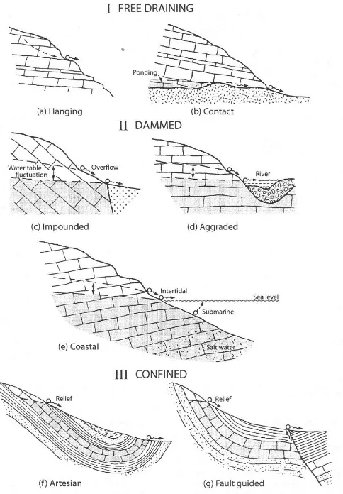
2.2.4. Groundwater discharge
Confined springs are impacted by impervious formations and/or fault planes, which may lead to ar-tesian conditions where groundwater is under positive pressure high enough that the piezometric potential reaches the ground surface.
[image:46.595.64.306.232.580.2]Groundwater discharge is linked to recharge and flow processes. Hence, the analysis of spring dis-charge, and in particular its recession, highlights information on recharge and flow. For example, a rapid recession of a spring hydrograph indicates limited storage of the aquifer (Friederich and Smart, 1982).
Figure 2.13: Type of karst springs (Ford and Williams, 2007).
2.2.5. Baseflow
1979) and characterised by a low-frequency phenomenon (Spongberg, 2000). An important aspect is the notation of a long-term change, hence originating from delayed sources (Hall, 1968).
Baseflow is one element that contributes to the shape of a stream hydrograph. Faster responding
contributions were referred to as ‘surface flow’ (Barnes, 1939), ‘overland flow‘ and ‘sub-surface
storm flow’ (Freeze and Cherry, 1979), ‘interflow’ and ‘direct runoff’ (Hall, 1968), or ‘overland flow’ and ‘interflow’ (Hiscock, 2014), for example. Accordingly, a stream hydrograph can be sub-divided into a baseflow component and other superimposed components. The contribution of baseflow to a stream ranges between a maximum (fully saturated basin) and a minimum (lowest recorded water-table configuration) (Freeze and Cherry, 1979).
The shape of a baseflow hydrograph may exhibit sharp rises, but there is always a very conspicu-ous time-lag between the storm input and the baseflow response (Barnes, 1939), with the general agreement that the shape of the recession follows an exponential decline (Maillet, 1905), valid for periods of no recharge (Hiscock, 2014). However, the baseflow component may also be approxi-mated by the combination of linear or linear and non-linear curves (Hall, 1968).
The concept of a delayed, low-flow groundwater-fed baseflow component of the total stream hydro-graph applies similarly to karst spring hydrohydro-graphs, which are sustained by discharge of diffuse (slow) flow into the conduits (White, 1988). In fact, Forkasiewicz and Paloc (1967) were the first au-thors that decomposed a karst spring hydrograph into three different superimposed components, each representing a different conceptual flow draining the aquifer. During the recession of a karst
spring, once the level of ‘pure baseflow’ is reached, the discharge can be linked to the drainage of the phreatic zone without any recharge or influence of rainfall occurring (Mangin, 1975). In drawing explicit parallels to surface hydrology, Atkinson (1977) interpreted the baseflow component of karst springs as the contribution from the narrow fissures, as opposed to the quick-flow assigned to the conduit domain. Since then, in the context of karst spring hydrography, the baseflow component has been interpreted as contribution from the low-permeability domain (Geyer, et al., 2008a), which justifies recession analysis in the context of coupled karst groundwater recharge, flow and dis-charge studies.
In this study, the baseflow component is referred to as the delayed response and low-flow compo-nent stored in the fissure openings a karst aquifer. During baseflow conditions, such low-flow com-ponent is drained into domains of larger permeability within the aquifer, e.g. into a conduit as illus-trated in Figure 2.6.
In this study the term ‘baseflow’ is replaced by the term ‘low-flow’ to avoid confusion with surface
2.2.6. Submarine and intertidal groundwater discharge (SiGD)
Groundwater discharge from coastal aquifers is grouped as intertidal discharge and/or SGD (Figure 2.13), where the combination of flows is summarised as submarine and intertidal groundwater dis-charge (SiGD).
Taniguchi, et al. (2002) pointed out the ambiguity of ‘older’ SGD definitions in which the considera-tion of re-circulated seawater wasn’t always clearly considered. For that reason, the same authors defined SGD as the sum of submarine fresh groundwater discharge and recirculated saline ground-water discharge, or, alternatively simply as the “mass transfer of groundwater across the sea floor”
(Zekt︠s︡er, et al., 2007).
In Ireland, SGD has been known from ancient times, mainly associated with karstic limestones (Zekt︠s︡er, et al., 2007). Important submarine and intertidal springs are known to drain the Gort Low-lands at Kinvara, or the northern and western part of the Burren Plateau. Further, the bay of Bell Harbour receives discharges from submarine and intertidal springs; the intertidal springs commonly emerge from enlarged joints, successively higher outlets becoming operative with higher flows (Drew, 1990). While many locations of intertidal springs are known, the discharge locations of purely SGD off the shore are more difficult to locate. SGD is presumably linked to lower sea levels during the Pleistocene (Drew, 1990). For example, the link between present SGD and formerly lower sea level during which the today’s SGD locations formed the principal outlet of an aquifer are well documented for the Mediterranean region where stacked karstic drainage networks have de-veloped resulting from changes in the sea level that have occurred since the end of the Miocene (Fleury, et al., 2007a).
The quantification of SiGD is difficult because their outlet cannot be physically captured / monitored as in the case of onshore springs. Therefore, for measuring or estimating SiGD of coastal aquifers, alternative (i.e. indirect methods) must be applied, such as:
a) measuring the seepage flow rate using seepage meters (Carr and Winter, 1980; Corbett, et al., 2003) or multi-level onshore piezometers (Freeze and Cherry, 1979; Taniguchi and Fukuo, 1996);
b) applying mass-balance approaches using natural geochemical tracers such as electrical conductivity (EC), short-lived radium isotopes, i.e. 222Ra, 223Ra, 224Ra, 226Ra, or oxygen-18
(δ18O) and deuterium (δ2H) (Moore, 2006; Peterson, et al., 2008; Santos, et al., 2008; Cave and Henry, 2011; Lee, et al., 2012; Null, et al., 2014; Knee, et al., 2016);
c) applying water balance approaches based on upon the contributing catchment (Sekulic and Vertacnik, 1996; Smith and Nield, 2003);
e) using numerical modelling (Thompson, et al., 2007; McCormack, et al., 2014; Taniguchi, et al., 2015); or
f) applying thermal imaging from remote sensing (Johnson, et al., 2008; Wilson and Rocha, 2012; Tamborski, et al., 2015).
While methods a) to e) can be considered as quantitative, method f) will only yield a purely qualita-tive result.
The abovementioned methods, however, all have limitations. Manual seepage meters in coastal environments are very labour intensive while the use of piezometric data (from multi-level nests), requires estimates of the aquifer hydraulic conductivity to calculate the groundwater discharge. The latter method implies practically a homogeneous lithological medium and Darcian flow – which is not the case in the context of karst, as discussed previously.
Distributed numerical modelling requires data on the spatial and temporal variation of boundary conditions, which is very difficult to obtain in reality (Taniguchi, et al., 2003).
Furthermore, most groundwater flow models are based on the assumption of constant fluid density, which may not be the case in coastal environments where the interface between fresh and saline groundwater is highly dispersed. In most coastal aquifers, this is, however, not the case (Zekt︠s︡er, et al., 2007).
The extraction of the baseflow component of streamflow hydrographs can only be applied to catch-ments that are drained by surface water and therefore generally not particularly suitable for karst catchments.
The use of remote sensing data seems to be limited to a qualitative SGD estimation, rather than a quantitative one, by estimating the temperature variations (Taniguchi, et al., 2003) or the salinity (Elachi and Van Zyl, 2006) on the sea water surface.
In Ireland, several studies have assessed the dynamics of local intertidal and submarine springs. Cave and Henry (2009) used a tidal prism model to estimate the SGD in Kinvara Bay. Between No-vember 2006 and June 2007, the average discharge was estimated at 22 m3/s, with maximum
rec-ords reaching 200 m3/s. Following this work, Cave and Henry (2011) quantified SiGD for the
Using the same approach of Cave and Henry (2009), Perriquet, et al. (2012) and Perriquet (2014) calculated a water balance for the catchment of Bell Harbour by estimating an upper limit (Eqn. 2.11) and lower limit (Eqn. 2.12) of SiGD by,
Q = 1 - (SHW–SLW)/33.5 x (HHW-HLW) x surface area Eqn. 2.11
Q = 1 - (SHW–SLW)/max. salinity flood tide x (HHW-HLW) x surface area Eqn. 2.12
with the average of salinity 𝑆𝐻𝑊− 𝑆𝐿𝑊 and the difference of height between high tide and low tide
𝐻𝐻𝑊− 𝐻𝐿𝑊. The authors used electrical conductivity (EC) records collected from one sampler
lo-cated in the middle of the bay at 1 m below sea level (mbsl). For the periods 02 Dec 2011 to 24 Jun 2011, 28 Mar 2012 to 07 Dec 2012 and 23 Dec 2012 to 28 Aug 2013, Perriquet (2014) estimated a mean SiGD of 4.9, 4.45 and 4.05 m3/s, respectively.
2.2.7. Quantifying groundwater flow dynamics in a well or borehole
Boreholes or wells can be used to infer local information on groundwater flow dynamics.
Different methods have been applied to study groundwater flow velocities within boreholes includ-ing high sensitivity impeller flow meters, electromagnetic flow meters and heat-pulse flow meters (Molz, et al., 1989; Molz, et al., 1994; Paillet, 2004; Busse, et al., 2016). However, deployment of the previously mentioned technologies depends on different conditions. For example, as summa-rised by Stowell (2013), all the above methods, with the exception of the heat-pulse flow meter, can be applied to cases where the vertical flow velocity exceeds 4 m/min. Another way of evaluating groundwater flow velocities in boreholes is done using distributed temperature sensing using opti-cal fibre cables (Read, et al., 2014). A more simple approach in assessing groundwater flow direc-tions and zones of inflow and outflow is by the use of single borehole dilution tests (SBDT) (Mau-rice, 2009).