Improved sorting networks with O(log n) depth

Original citation:

Paterson, Michael S. (1987) Improved sorting networks with O(log n) depth. University of Warwick. Department of Computer Science. (Department of Computer Science

Research Report). (Unpublished) CS-RR-089

Permanent WRAP url:

http://wrap.warwick.ac.uk/60785

Copyright and reuse:

The Warwick Research Archive Portal (WRAP) makes this work by researchers of the University of Warwick available open access under the following conditions. Copyright © and all moral rights to the version of the paper presented here belong to the individual author(s) and/or other copyright owners. To the extent reasonable and practicable the material made available in WRAP has been checked for eligibility before being made available.

Copies of full items can be used for personal research or study, educational, or not-for-profit purposes without prior permission or charge. Provided that the authors, title and full bibliographic details are credited, a hyperlink and/or URL is given for the original metadata page and the content is not changed in any way.

A note on versions:

The version presented in WRAP is the published version or, version of record, and may be cited as it appears here.For more information, please contact the WRAP Team at:

Research report 89

IMPROVED SORTING NETWORKS WITH

O(LOG N) DEPTH

M S Paterson

(RR89)

Abstract

The sorting network described by Ajtai, KomlOs and Szemeredi was the first to achieve a depth of O(Iog n). The networks introduced here are simplifications and improvements based strongly on their work. While the constants obtained for the depth bound still prevent the construction being of practical value, the structure of the presentation offers a convenient basis for further development.

IMPROVED SORTING NETWORKS WITH 0(LOG N) DEPTH

M.S.Paterson

Department of Computer Science University of Warwick Coventry, CV4 7AL, England

Abstract

The sorting network described by Ajtai, Komi& and Szemerall was the first to achieve a depth of

O(log n). The networks introduced here are simplifications and improvements based strongly on

their work. While the constants obtained for the depth bound still prevent the construction being of

practical value, the structure of the presentation offers a convenient basis for further development.

1. Introduction

We consider networks which are constructed using components of a single type, the

comparator. A comparator has two inputs and yields as its two outputs the input elements in

sorted order. The N inputs are presented on N wires and at each successive level of the network

at most N/2 disjoint pairs of wires are put into comparators. After each level the N wires carry

the original elements in some permuted order and the network is a sorting network if the

elements are always in sorted order after the final level of comparators. The depth of a network is

just the number of levels.

One very simple regular sorting network, "odd-even sort", has depth N for N>2. An elegant

recursive network due to Batcher [3] requires only about (log N)2/2 depth. A useful source for

background and references in this area is [6]. The familiar S2(N log N)-comparisons lower bound

for sorting immediately gives an Sl(log N) lower bound for the depth of sorting networks.

Following the appearance of [3] in 1968, a longstanding open problem has been to close this depth

complexity gap. This was finally achieved in 1983 by Ajtai, Komi& and Szemeredi [2]) with

a sorting network of O(log N) depth. Their construction and proof are of some intricacy and since

their main concern was just to provide an existence proof for such networks the numerical constant

which allows a more accessible proof. The constant obtained in our proof is still so large that

Batcher's network has less depth for all practical sizes of networks, but we have some hope that

further refinements may yield a substantially improved constant.

The sorting network described here was originally presented at the Complexity Theory meeting in

Oberwolfach in October 1983 and again at Theory Day at Columbia University in March 1984. I

would like to thank Pippenger, Rackoff and Skyum for valuable discussions during visits to

Aarhus University and IBM San Jose in 1983, and Cole for useful comments on a preliminary

draught of this paper. I also acknowledge the patient urging of many colleagues without whom this

work would have remained in oral tradition, and the support of the Science and Engineering

Research Council with a Senior Fellowship from 1985.

2. Overview of network

Consider a binary tree with 'bags' at each node. Initially the set of N elements to be sorted is

contained in the single bag at the root. Suppose we were to partition the elements from the root bag

into a left and a right half, and we transferred these to the left and right daughter bags respectively.

(We shall use the terminology of left and right rather than small and large in the sorted order of

elements to accord with a geometrical picture of a binary tree with the root at the top and branches

going down to left and right.) If we were to continue in the same way then after log N stages the

elements would have been sorted. Unfortunately the task of partitioning a set of n elements into

left and right halves requires 52(log n) levels of comparators. The idea used by Ajtai, Komi& and

Szemeredi [2]) is to take an approximate partition of elements, which can be achieved in only

a constant number of comparator levels, but to introduce some error-recovery structure into the

sorting scheme. In our most basic scheme this is done by partitioning the bag of elements at each

node into four parts: the main left and right 'halves', which are sent down to the daughter bags, and

in addition two small fragments from the extreme ends of the partitioning process, which are

intended to include most of the elements that were wrongly routed from higher in the tree and

which are now returned to the parent bag above. Our network operates almost uniformly in this

and this size increases in a geometrical progression with the depth of this level below the root. The

upper smaller bags of the tree are concerned with recycling that small fraction of the elements which

may have been misclassified in some partitioning process. As time progresses the size of each bag

is reduced, again in a geometric progression, thus 'squeezing' the elements down the tree towards

their final locations at the leaves. The correctness of the network is demonstrated by proving an

invariant which bounds the proportion, within each bag, of elements with any particular degree of

displacement from their 'proper' positions. The notion of 'strangeness' used in this invariant is a

simplification of that introduced in [1]. During the account below of the network and the

correctness proof, various parameters are required. At each point we set out the inequalities which

the parameters have to satisfy and produce an example of suitable parameters in order to animate the

description.

We initially describe the sizes of various sets of elements as if they were real numbers. Ultimately

we will show how appropriate integer values can be chosen so that the required inequalities still

hold.

3. Definitions and building blocks

In [1] the notion of an a-halver is introduced. For any a > 0, an E-halver for m elements is a

comparator network with m inputs, and with outputs partitioned into a left and a right block each of

size m/2. The E-halver has the property that, for any set of inputs and any k 5 m/2, the number

of elements from the k leftmost in the ordering which are output in the right block, and from the k

rightmost which are output in the left block, are each less than Ek. An e-halver can be constructed

in constant depth (depending on E), for example by using expander graphs. This is described in

[1], but where those authors go on to build "E-nearsorts", we shall use the more limited component

which is described immediately. A (X, E, a0)

-

of its m input values into four parts FL, CL, CR, FR, of sizes Xm/2, (1

—

Xm/2 respectively. The set FL (for "far-left") has the property that for any k, k Xm/2, the

number of elements from the set of k leftmost input values which are not in FL is less than Ek.

m/2, the number of elements from the set of k leftmost input values which are not in FL or CL

("centre-left") is less than eok, and similarly for elements from the right half of the ordering which

end up not in FR or CR. It is easy to build some (X, E, e0)-separator from a constant number of

eo-halvers. In particular if we use an eo-halver on the m inputs, then apply an eo-halver to each

of the resulting output sets of size m/2, then two eo-halvers to each extreme set of size m/4 and

so on through p levels, the resulting network yields a (2-1)+1, pep, E0)-separator. The p levels of

halvers produce a sequence of 2p blocks. The extreme blocks are taken for FL and FR, while

the left and right halves of the remaining sequence are combined to form CL and CR

respectively. To verify the value of a we note that a proportion eo of some set of extreme

elements may escape to the 'wrong' output block at each of the p layers of eo-halvers.

INPUT

0 halv

Fig. 1. Construction of a (1/8, a, co)-separator from a sequence of eo-halvers

(i) For sample parameters we will take: p = 4, X = 1/8, E0 = 1/72, and

a =

At various places in our construction we want to sort sets of a small constant size. It is convenient

to use there the sorting network due to Batcher [3], the depth of which for m elements is

b A

-4

°lA Cs'l

W-b

CD

\

4. The network

The sorting network is structured about a complete binary tree which we shall imagine with the root

at the top and leaves below. Associated with each node of the treee is a bag which contains a

number of the elements being sorted. The capacity of a bag is the maximum number of elements

which can be stored in that bag. For most of the algorithm each bag is either empty or filled to its

capacity. With the root considered to be at level 0 in the tree, the capacity of each bag at level d

is r.Ad for some constant A, and some value of r decreasing with time.

(ii) For example: A = 3.

/

\. / \,.

/

\. / '\.

Fig. 2. Tree structure of bags.

Special situations occur at the topmost and lowest nonempty levels of the tree so we start with a

description of the sorting process at intermediate levels. The algorithm works in stages beginning

at stage 1. At odd stages all the bags at odd levels are empty and the bags at (some) even levels are

full, while the opposite holds at even stages. At each stage the elements in any full bag are

partitioned by a separator, the far-left and far-right parts are sent up to the parent bag and the

Stage t

E55,

(1-20 b/ ( 2A)

Stage t+1

capacity b

capacity v b < b

XbA

X bA

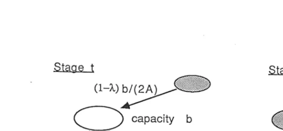
Fig. 3. Reduction of bag capacities after each stage.

Consider a bag, empty with capacity b at the beginning of some stage which is filled to its new

capacity vb at the end of the stage. Thus:

vb = 2XbA + (1-X)b/(2A).

We require v < 1 so that the capacities diminish at each stage and elements are squeezed down the

tree in the course of the algorithm, i.e.

(1) v = 2XA + (1-X)/(2A) < 1

(iii) With our sample parameters: v = 43/48.

The capacity of each bag at level d after stage t will be c•vt-Ad for some constant c.

To each bag there corresponds naturally an interval within the sorted order of the elements. The

root bag corresponds to the whole ordered set, its left and right daughter bags correspond to the left

and right halves of the ordering, and, for example, the bag reached by taking the path LRL down

from the root corresponds to the third eighth from the left. To work out the strangeness of some

element in a particular bag we count the number of steps up the tree from that bag towards the root

which are needed to arrive at a bag within whose natural interval the element lies. Thus:

(i) all elements in the root bag have strangeness zero;

(ii) the strangeness of any element if nonzero is decreased by one if the element is sent up to

(iii) when any element is sent down to a daughter bag its strangeness increases by one,

except only when its strangeness is zero and it is sent down to the 'correct' daughter in

which case its strangeness remains zero.

For any bag B and integer j > 0, we define Si(B) at some time to be the number of elements

currently in B with strangeness j or more, expressed as a proportion of the capacity of B. The

invariant that we maintain in order to assure the correctness of our construction is that:

(2) Si(B) < p..5j-1 for all B and for all j 1.

(iv) For example, p. = 1/36, 5 = 1/40.

In [1] the authors' concern was solely with an existence proof and they use corresponding

parameters p. = 10-74,

S = 10-6.

At each stage the elements in each bag are partitioned by a (X, c, 80)-separator, the parts FL and

FR are sent up to its parent; CL and CR are sent down to its left and right daughter respectively.

Assuming that (2) held at the previous stage we can give an upper bound on the number of

elements of strangeness j or more in some bag B at the following stage. Suppose the new

capacity of B to be vb and the old capacities of B's parent bag and daughter bags to be b/A and

bA respectively. For j >1 the elements of strangeness j or more that find their way into B are

either elements of strangeness j+1 or more from the daughter bags, or elements of strangeness j-1

or more which are sent down the wrong way by the parent bag. If we ensure that the FL and rR

parts of the separator are each sufficiently large to accommodate any elements of positive

strangeness then only at most a proportion c of these are sent down. We therefore require that:

(3) X/2.

Then the new strangeness of B, S'i(B), satisfies:

S'i(B)-vb < 2bA1.15:1 (b/A) 4-2 for j >1.

To ensure that (2) holds for the new stage we will choose parameters satisfying:

(4) 2A252 + vAS.

Proving the required bound for S'1(B) is more complicated. The first term, 2bA IA, appears just

as before, representing the import of elements of strangeness two or more from B's daughters.

Now however, some elements are misdirected downwards to B by B's parent not only because

of mistakes by the separator but also because the parent bag may contain too many of the elements

appropriate to B's sister, C say. Let this set of elements of strangeness zero with respect to C be

denoted by V. The 'natural' location for V would be the whole contents of the subtree rooted at

C together with one half of the contents of B's parent, one eighth of her greatgrandparent, and so

on, assuming for the present an infinite chain of ancestors. The sizes of the bags will be such that

V would fit exactly in this space. In reality some elements of V may have been displaced from

this area and so might be occupying more than half of B's parent's bag.

b/(8A 3)

The bag of a daughter of C may contain up to S2bA elements from outside V. A bag two levels

further down the tree may contain S4bA3 such elements, and so on. The total number of elements

thus intruding into V's area in levels lower than B is at most

2S2bA + 8S4bA3 + 32S6bA5 + < 2p.8bA/(1 — 452A2).

The area above B's parent appropriate to V may in fact contain no elements of V. The total space

here amounts to

b/(8A3) + b/(32A5) + = b/(8A3 — 2A).

In addition B's parent may contain up to S 1b/A ( < p.b/A ) strangers.

Thus, even if the initial halving of B's parent were done perfectly, a surplus of elements of V and

other strangers with respect to B may spill across into B. The surplus is bounded by the sum of

the three terms identified immediately above. Splitting error adds a further term of be..0/(2A) since

up to that number of elements may be misplaced in the initial split. Thus we have:

S'i(B).v < 2p.8A + 2p.8A/(1 — 462A2) + 1/(8A3 — 2A) + WA + e0/(2A).

Since we require S' 1(B) < p., our parameters must satisfy:

(5) 2p.8A2 + 2µ8A2/(1— 452A2) + 1/(8A2 — 2) + µ + vp.A

(vi) The choice Eo = 1/72 suffices since 1/80 + 5/391 +1/70 + 1/36 + 1/144 < 43/576.

5. Boundary situations

During the course of the algorithm the elements migrate down through the tree. We will arrange

that there is at most one partially filled level. Above this, the levels are alternately empty and full as

already described; below, all levels are empty. To this end we require that at this partial level

each separator should send up to its parent bag the normal number of elements if it has sufficiently

many. After this requirement is met, any remaining elements can be sent down to the daughter

bags in equal numbers. Since the strangeness bounds are expressed as a proportion of bag capacity

rather than as a proportion of the elements present, it is easy to satisfy these bounds at the partial

level. To ensure that no more than the permitted number of elements with a certain strangeness are

sent down, it suffices to adapt the usual separators in the following manner. After the initial split

each half. The virtual elements added to the left half are always 'more right' in comparisons with

existing elements of the left half, whereas the virtual elements of the right half are 'more left' than

the real elements of that half. The modified separator is obtained by deleting from the usual

separator all of those comparisons involving virtual elements and routing the real elements

appropriately. If this results in any virtual elements reaching FL or FR then they should now be

replaced by arbitrary real elements from CL or CR respectively.

We must check that the strangeness invariants are satisfied around the partial level. For S' 1, the

initial split will leave no greater number of the elements than usual in the 'wrong' half, though the

proportion of these elements may be greater. For j >1, the introduction of the virtual elements

into each half serves only to assist the strange elements into parts FL and FR, and the number of

strange elements sent down will not be excessive.

The other abnormal boundary level is at the root of the tree. Here we would like the root node to

behave as if it were an ordinary interior node of the tree. We therefore keep above it a subset of

the elements, the cold storage, with which the root exchanges elements as with a parent. No

comparisons are required within the cold storage, and the strangeness invariants are satisfied at the

root since by definition all elements have strangeness zero there. The arguments in Section 4

involving an infinite chain of ancestors carry through if we regard the cold storage as simulating

half the root's parent, one quarter of her grandparent, and so on. The capacity of the cold storage

is therefore to be:

r/(2A) + r/(8A3) + = 2Ar/(4A2 — 1) at even stages,

and: r/(4A2) + rA16A4) + = r/(4A2 — 1) at odd stages,

where r is the capacity at the root. To begin the algorithm N(1-1/(4A2)) of the input elements

are placed in the root bag and the remaining N/(4A2) elements are considered to be the cold

storage.

6. Final stages

stage, when all the odd levels are empty, the number of elements in a bag at level 2j which are in

the wrong half of the tree is bounded above by:

rA2iS2i < rA2igS2i-1 rA21.1.8

provided we have:

(6) A8 1.

Therefore this number of elements is less than one, i.e. zero, by the time r has been reduced to

1/(A2p.S).

(vii) We have AS = 3/40 1 and the critical value of r = 1/(A2p.S) = 160.

At such a time then, there are no elements in the wrong half of the tree, so we exactly separate the

set of all elements in the root bag and the cold storage into a left and a right half. From these halves

the root and cold storage for each subtree can be immediately formed. To achieve the exact

separation for a set of bounded size a Batcher sorting network [3] may be used. From this stage on

a new root-splitting step will be required at regular bounded intervals, resulting in a rapidly

growing forest of independent subtrees. Finally, when these subtrees reach a conveniently small,

bounded size, each can be exactly sorted to give the final result.

To estimate the total number of stages required by the algorithm, we note that the bags at level

log N are initially of capacity e(N-Alog N), where our logarithms are to base 2. At the last stage

of the algorithm these bags are of capacity 8(1), since they are within a bounded number of levels

of bags of bounded capacity. Thus the number, k, of stages of the algorithm satisfies:

N-A10g N.vk =

i.e. k = log2N.log(2A)/(-log v) + 0(1).

(viii) We have: log(2A)/(-log v) = (log 6) / log (48/43) < 17.

7. Integer rounding

In previous sections we have specified the 'ideal' sizes of various sets of elements as real numbers

and it remains to show how to pick integer sizes satisfying all the constraints. Provided that the

sizes chosen are all very close to the ideal sizes and that the capacities of all the bags are sufficiently

the strangeness bounds are expressed as a proportion of the capacity of a bag the possibly small

actual sizes at the partial level cause no special difficulty. The smallest capacities in our algorithm

arise at the root of a tree when we are about to split the tree. (For example, in Section 6 the critical

root capacity was given as 160 for our parameters.) In case the corresponding value for some

choice of paramaters is too small to absorb the effects of rounding, the root-splitting may be done at

an earlier stage. Referring to Section 6, we see that no elements at or below level 2j are in the

wrong half of the tree provided that:

r

At an odd stage the number of elements above level 2j is about r(2A)2i/(4A2 — 1). If we use

Batcher's method to sort exactly this set of elements (instead of just the root bag and cold storage)

then the tree can be properly split. For all of the networks we describe later, j = 2 suffices.

(ix) With A=3,11=1/36, 8=1/40, j=2, we could maintain r > 28,000 by sorting sets of size about

one million.

It is convenient and efficient for the design of separators that the actual number of elements in each

bag be even. Note that this can be achieved even when N is odd because of our use of cold

storage. We provide a simple recipe for the integer sizes of the bags which will ensure that these

cannot stray far from their ideal sizes. Each ideally empty bag is actually empty. For each subtree

rooted at a non-empty node, if the ideal total content of the subtree is a, then the actual content is

to be 2

[a/21.

a,

while the ideal contents of its granddaughter subtrees are

p.

bag at that node are b and Z(b) respectively then:

b = a — 413, Z(b) = 2

Fa/21 -

Fp/21,

Since only the partial level of bags can ever become very small there is no difficulty in maintaining

the relationship. Thus Z(b) is even and the close agreement between b and Z(b) satisfies our

requirements.

We shall see that our ideal (X', c, c0)-separator, with say X' = 2-P+1, can be refined to take

account of integer sizes and to allow the size of FL and FR to be arbitrary within the range

sufficiently small that our algorithm with parameter X, say, never requires the size of FL or RL

to be less than 2 1Z(b)/2. Suppose that some full bag has ideal capacity b and the ideal content for

the corresponding subtree is a. Our recipe specifies:

IFLI = IFRI = ra/21— [(a — 2 b)/21 >

Fa/21 -

X2(b)/2 < X'(

Fa/21

a/2 +

and so it suffices to have:

X X' + 2/b.

In the interests of clarity we ignored this consequence of rounding in our earlier description and

identified X and X', but now values for X and v must be increased appropriately. The effect on

our final constant depend on the minimum size of b.

(x) With b 160 and X' = 1/8, we need X. 0.1375, and when v increases correspondingly

the number of stages more than triples. However with b 28,000 the increase in the number of

stages is less than 0.5%.

The principal motivation for making the sizes of bags even numbers is to simplify the analysis of

halvers and to permit the relatively clean bound of the theorem in the next section. This is of

significance only for the initial (symmetrical) halver step in our separators. The later halving steps

are not applied to sets of even size but these can be dealt with by introducing a 'virtual' element as

described below. Were this done in the first step also, it would degrade the performance

unacceptably for small values of k.

Consider a halver which is on the left side of the separator structure and whose function therefore is

to ensure, for some c and for some range of values of k, that fewer than ek elements from the

extreme left k of its input elements are output in the right (i.e. wrong) half. If the number of input

elements is 2n — 1 we introduce a new 'virtual' element which is considered to be to the right of

all the real elements. After the application of a 'standard' halver for 2n elements, the virtual

element will have been output to the right and is discarded. The specifications for the standard

halver will have the same value of

c

Finally we note that whenever the size of FL and FR has to be increased to achieve the specified

bag sizes we can transfer elements arbitrarily from CL to FL and from CR to FR without

worsening the error bounds.

8. Separators and constants

We prepare for a more economical construction of separators by generalising the notion of halver

which we defined in Section 3. For any c > 0 and a, 0 < a 1, an (e, a)-halver for m=2n

elements is defined in the same way as an c-halver except that the key property is only required to

hold for sets of size k with k 5_ an instead of for all k 5 n. We shall see that this less stringent

requirement allows a considerable economy in depth when a << 1.

Theorem For 0 < e 1a, 0 < a 5_ 1 and n > 0, there exists an (c, a)-halver for 2n elements

with depth C(a,c) where:

C(a, c) = I1 + (h(ca) + h((1-c)a)) / (-ca ln((1-c)a))1, and:

h(x) = -x In x — (1-x) In (1-x).

The proof of this theorem is given in the Appendix. An essential feature of the above result is that

an explicit depth is given which holds for all values of n. Previously published results such as [4]

give just asymptotic values as n tends to infinity. Since our halvers are to work synchronously at

all levels of the tree and since the root level is small for a significant proportion of the stages, this

stronger result is necessary. We have, however, taken a slightly larger value for C than that given

by the asymptotic bounds in order to simplify our analysis. Our proof does not yield an explicit

halver network; all currently known explicit constructions require a much greater depth. See

references [8], [5], and [7] for further information and recent work.

An easy analysis reveals that, when c --> 0:

C(1, e) --> -21n e / e,

while for fixed cc, 0 < cc < 1:

The total depth of the network we have described is approximately

log2N.p-C(1, 60).log(2A)/(-log v)

when we construct a (2-P+1, 13E0, 6.0-separator using p levels of 60-halvers.

(xi) Our sample parameters p=4, X.'=1/8, 60=1/72, A=3, p:=1/36 and 5=1/40 yield a value that is

just under 50,000 log2N.

It is possible to do a little better just by varying the parameters. For example we have found that

the values p=4, 2'=1/8, 6.0=3/223, A=2.7, p.=1/16 and 5=1/34 can reduce the constant below

30,000. However we shall show next how this constant may be more substantially improved after

a closer analysis of separators.

The error estimate E is the sum of error contributions from each of the p levels. Suppose we

allow an error of ei at level i for i = p, where e = el + 62 + + cp. In the coarse analysis

we used until now we adopted the pessimistic setting of a = 1, and have used a halver of depth

C(1, ei) at level i. Referring to figure 1 again, we see that at level i the ratio of the number of

strangers to the size of a half is at worst (p. : 1/2i) so that we could actually construct a separator

with total depth

C(211, el) + C(4p., 62) + + C(2131.1., 6,p).

Note that our constraints ensure that 21)1.1. 5 1.

For the 60-bound that also has to be assured by the first-level halver, we can again improve on the

naive estimate of a =1. Referring back to the derivation of the bound on S'1 in Section 4, we see

that the number of elements of V in the bag of B's parent is at most

b(1 +1.1)/(2A) where ri = 4µ6A2/(1— 452A2) + 1/(4A2 — 1).

In addition there may be up to Sib/A strangers. Since all but a proportion E of 'right' strangers

would get sent up the tree with FR, the worst case in the estimation of S'1 is when there are

b.t/A strangers and they are all to the 'left'. (This case can arise only when B is the right (left)

daughter of a right (left respectively) daughter. In the situation shown in figure 4 any elements

with strangeness exactly one for B's parent must be 'left' strangers. Taking account of this

number of good elements (i.e. those appropriate to B) in this bag is only b(1 — — 2p,)/(2A), and

so to limit to 60/(2A) the further influx of strangers to B due to good elements being sent the

wrong way the first level halver only requires depth C(1 — rl — €0) instead of our former

estimate of C(1, 60). The total depth needed for a separator is now reduced to

max( C(2p., E1), C(1 — 2 t, 60) ) + C(411, 62) + + C(2Pp,, cp).

With this more refined construction the parameters

p=4, 2C=1/8, A=2.7, p.=1/20, 8=1/40, F. 0 = 1 / 5 9 , 61=1/134, 62=1/85, 63=1/83, 64=1/62

yield a constant below 6500. This comes from a network with about 9.5 log2N stages and

separators of depth 678. The best constant we have found is under 6100 and achieved using

parameters given approximately by:

p=5, A=4.75, ..i=1/50, 8=1/57, and for i=0,...,5, 1/6i = 62, 199, 110, 109, 106, 90,

to yield a network with about 6.15 log2N stages each of depth less than a thousand.

9. Ideas for improvements

When we classify the contents of a bag we must expect a small proportion of elements from the

middle range of values to be misclassified between CL and CR so that they are sent down to the

wrong daughter bag and acquire strangeness 1. A more cautious classification would produce a

borderline class which was to be retained in the same bag at the next stage. The emptiness at

alternate levels in the construction described above was a convenient simplification but is not an

essential feature. To incorporate the modifications suggested in this section all the bags above a

certain level in the tree are maintained full to capacity. Consequent changes are required at the

upper and lower extreme levels.

Consider the extreme left elements which may be found in a bag at a left daughter node in the tree.

It will be clear that if these elements need to be moved left and have nonzero strangeness then they

must have strangeness at least two and could usefully be sent up two levels at once. Similar

reasoning holds for extreme right elements in a right daughter bag.

the progress of correctly sorted elements down the tree towards the leaves. The constraints on the

parameters are easily handled but the technology of producing efficient classifiers of the more

complicated forms which are required becomes much more intricate.

10. Conclusion

We have tried to describe these depth 8(log n) sorting networks as cleanly as possible. The

constraints on the parameters have been extracted as a simple set of inequalities. While the

numerical bounds we have proved suggest that the present construction is still far from efficient,

we hope that the framework presented will encourage further progress towards a practical

algorithm.

Open Problem Develop an error analysis which measures more closely the performance of this

kind of sorting network.

Conjecture The depth of network required for the correctness of our algorithm is overestimated

hugely by our analysis.

References

[1] M. Ajtai, J. Komi& and E. Szemeredi, "An 0(n log n) sorting network," Proc. 15th Ann.

ACM Symp. on Theory of Computing (1983) 1-9.

[2] M. Ajtai, J. Komi& and E. Szemeredi, "Sorting in C log N parallel steps," Combinatorica 3(1983) 1-19.

[3] K. Batcher, "Sorting networks and their applications," AFIPS Spring Joint Computer

Conference 32(1968) 307-314.

[4] F. Chung, "On concentrators, superconcentrators, generalizers, and nonblocking networks,"

The Bell System Technical Journal 58,8(1978) 1765-1777.

[5] 0. Gabber and Z. Galil, "Explicit constructions of linear-sized superconcentrators," J.

Comp. Sys. Sci. 22(1981) 407-420.

[6] D.E. Knuth, The Art of Computer Programming, Vol.3, "Sorting and Searching" (Addison-Wesley 1973).

[7] A. Lubotzky, R. Phillips and P. Sarnak, "Explicit expanders and the Ramanujan conjectures," Proc. 18th Ann. ACM Symp. on Theory of Computing (1986) 240-246.

[8] G.A. Margulis, "Explicit constructions of concentrators," Problemy Inf. Trans. 9(1973) 325-332.

Appendix (Proof of Halver Theorem)

Theorem For 0 < e 1/2, 0 < a .5 1 and n > 0, there exists an (E, a)-halver for 2n elements

with depth C(a, a) = [G(a, e)1 where:

G(a, e) = 1 + (h(ea) + h((1-e)cc)) / (-ea ln((l-e)a)), and:

h(x) = -x In x — (1-x) In (1-x).

Proof We shall describe the halving networks in terms of comparison algorithms using storage

registers and compare-and-exchange operations on pairs of these registers. This is an equivalent

model to that with wires and comparators used above. The registers are divided into equal sets A

and B with n registers in each. At every step of the algorithm, comparisons are made between

the contents of n disjoint pairs of registers, one from A and one from B. For each pair an

exchange is made if necessary so that the more 'left' value is put in the A-register and the more

'right' in the B-register. Suppose that the algorithm proceeds in this way for c steps and at step

i, 1 _5 i 5_ c, the set of pairs to be compared is given by the bijection gi : A— B, i.e. for all a E A,

registers a E A and gi(a) E B are compared. We will find that for c sufficiently large most of

the algorithms of this form satisfy our halving condition. The total number of distinct algorithms

with c steps is exactly (nOc. We calculate an upper bound for the number of such algorithms

which fail to be (e, a)-halvers.

Consider a failing algorithm Q and some set of inputs for which Q fails. Thus there is a k 5_ an

such that the set S of the k rightmost (or leftmost) input elements is badly distributed at the end

of the algorithm, i.e. some set X of A-registers (or B-registers respectively) of size r = Feld still

contains r elements of S. Since for any r we may as well choose k maximal subject to r = rekl

and k an, we can assume k = max ( Lr/e j , Lan] ). A sufficient set of pairs < r,k > to cover all

possible failing algorithms is given by:

R(n, E, CC) = < r,k > I 1 < r < ep, k = Lr/e j l< Fepi , p >) where p =

Lan j.

This follows from the inequalities:

Without loss of generality we consider the case X c A. It is clear that the contents of any

A-register can only become more 'left' as the result of an exchange, whilst B-A-registers become more

'right'. Therefore at the beginning of the algorithm X contained elements from S, and

furthermore every B-register compared with any register in X during the algorithm must have

also contained an element of S at the time and so will still do so at the end of the algorithm.

Denoting the whole set of such B-registers by Q(X), we have shown that:

I Q(X)Ik - r.

For any X c A with IXI = r, and Y c B with IYI = k - r, the number of bijections g : A -4B

such that g(X) c Y is

(k - r)! (n - r)! / (k - 2r)!

Taking into account the number of possible choices for r, X and Y, and the alternatives of X c A

or X c B, we obtain an upper bound for the proportion, P(c), of failing algorithms with c steps

of:

P(c) (rir) \k-r) (\k r) (nr))

c

<r,lc>e R(n,E,a)

(nr) (nk_r) OC-T)/I1) IC R (n, E, a)

We define h on the interval [0,1] by:

h(x) = -x In x - (1-x) In (1-x) for 0 < x < 1, and

h(0) = h(1) = O.

h is a familiar entropy function except that we find it more convenient here to use natural

logarithms. The approximation we shall use for binomial coefficients is given in the following

lemma.

Lemma For n > 0 and 0 < r < n,

ln(nr) < n•h(r/n) - 1/21n(min (r, n-r)) - 1/21n 7C.

Proof A result of Robbins [9] yields the following inequalities:

Hence for 0 < r < n,

ln(nr) — n-h(r/n) + 1/21n(minfr, n-r))

< -1/21n(max{r, n-r}) + 1/21n n — 1/21n 27c + 1/(12n) — 1/(12r+1) — 1/(12(n-r)+1). < -1/21n 7c. +

Now,

in (n r) (11/J ((k-r )/n)rel

< n{h(r/n) + h((k-r)/n) + cr/n• ln((k-r)/n)} — 1/21n r — 1/21n(min (k-r, n-k+r}) — In it

r ln((k-r)/n) — in r — In it since min {k-r, n-k+r} r,

provided we choose a value for c satisfying:

c 1 + (h(r/n) + h((k-r)/n))/(-r/n. ln((k-r)/n)) = G(k/n, r/k).

If we can choose c to satisfy this inequality for all values of r and k in the summation then:

P(c) < i_D(kn-r)r < 2 V k-r r R (n,e,a) R (n,E,a)

2fep1

< 2._(1+_L) <

7cn TC en

If en < 2 then P(c) < 1 follows immediately since r 2.

All that remains to be proved is that c = [G(a, e)1 is an adequate choice for c. Since all < r, k >

in R(n,

e,

that G(a, a) is an increasing function of a and a decreasing function of e.

Lemma For all 0 <a<_ 1, 0 < e < 1,

(i) awas < 0,

Proof

Let u = h(acc) + h((1-e)a), v = -ECG ln((l-e)a, and F = u/v. Then u,v > 0 and G(cc,$) = 1 + F.

Now,

Ev

= -Ea ln(Ea) + £0: ln(1-ca) — Ea ln((l-e)a) + ea ln(1-(1-c)a) — u — Fe2cc2/(1-E)

= acc ln(1-ca) + a ln((l-e)a) + (1-cc) ln(1-(1-E)a) — Fa2a2/(1-a)

< 0 for all 0 < cc 5 1, 0 < E < 1, and (i) is proved.

Similarly for (ii), if a 1/2,

av

= -ECC ln(ea) + ea ln(1-ea) — (1-a)a In((1-E)cc) + (1-e)cc ln(1-(1-e)cc) — u + Fea

= ln(1-ca) + ln(1-(1-e)cc) + F8CC

ln(1-acc) — h(ea)/1n(ea) + ln(1-(1-c)a) — h((1-e)a)/1n((1-E)a) since 1-c

> 0 since h(y) > In y.ln(1-y) for 0 < y < 1.

This inequality for h follows from the substitutions z = y and z = (1-y) in the simple inequality:

z > -(1-z) ln(1-z) for 0 < z < 1.