Nuclear magnetic resonance in some binary liquid systems showing a metal non metal transition

warwick.ac.uk/lib-publications

A Thesis Submitted for the Degree of PhD at the University of Warwick

Permanent WRAP URL:

http://wrap.warwick.ac.uk/106906

Copyright and reuse:

This thesis is made available online and is protected by original copyright.

Please scroll down to view the document itself.

Please refer to the repository record for this item for information to help you to cite it.

Our policy information is available from the repository home page.

copyright o f this thesis rests with \ts author.

V . .

This copy o f the thesis has been supplied

on condition that anyonç who consults it is

understood to recognise that it$ copyright rests

with its author and that no quotation from

the thesis and *no information derived* from it

may "be -published without the author’s prior

written consent

A

zynt/vi

.

REPRODUCED

FROM THE

BEST

LIQUID SYSTEMS SHOWING A METAL NON-METAL

TRANSITION

DAVID JOHN KIRBY, B.Sc.

eoo*: re

A thesis submitted to the University of Warwick

for admission to the degree of Doctor of Philosophy

t a b l e o f c o n t e n t s

ACKNOWLEDGEMENTS

DECLARATION

ABSTRACT

PAGE

CHAPTER ONE

THE METAL NON-METAL TRANSITION IN BINARY LIQUID SYSTEMS

1.1i Introduction 1

1.2: Bonding 6

1.3: Liquid Structure 8

1.4: Metallic conductors 10

1.5: The Pseudogap in Non-Metallic Liquids 12

1.6: Molecular Bond Model for Non-Metallic Liquids 18

1.7: Electronic Structure Away from Stoichiometry 21

• 1.8: The Effects of Correlation 25

CHAPTER TWO

NUCLEAR MAGNETIC RESONANCE

2.1: Magnetic Susceptibility 28

2.2: Introduction to Nuclear Magnetic Resonance 29

2.3: Resonance Shifts and Relaxation Data 34

2.4: Nuclear Resonance Shifts 39

2.5: Spin Lattice Relaxation 43

2.6: Investigation of Electronic Structure 47

CHAPTER THREE

EXPERIMENTAL

3.1: Sample Preparation 81

3.1.1: Caesium-Gold and Caesium-Antimony Alloys 51

3.2: D.C. Magnetic Field

3.3: The NMR Furnace

3.4: The NMR Pulse Spectrometer

3.5: Hie Sample Probe

3.6: Signal Processing

56 57 60 62 69 CHAPTER FOUR

THE CAESIUM-GOLD SYSTEM

4.1: Introduction 72

4.2: NMR in The Stoichiometric Compound CsAu 74

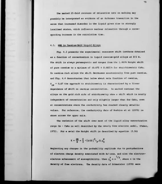
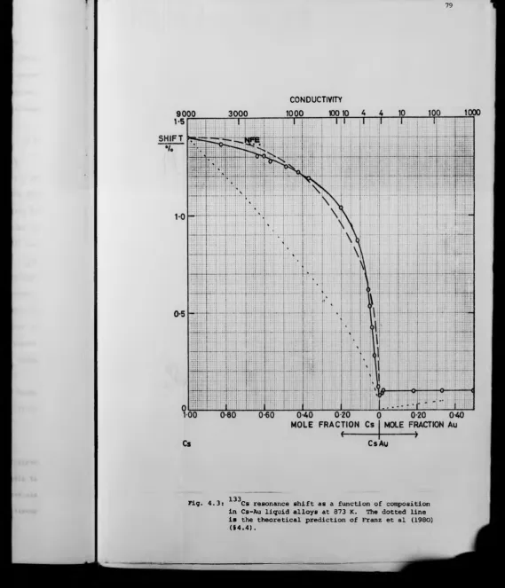
4.3: NMR in Caesium-Gold Liquid Alloys 78

4.4: Relation to Other Properties 90

4.5: Summary of the Caesium-Gold System 96

CHAPTER FIVE

THE CAESIUM-ANTIMONY SYSTEM

5.1: Introduction 99

5.2: NMR in Caesium-Antimony Liquid Alloys 102

5.3: NMR in the Stoichiometric Compounds Cs^Sb and CsSb 111

5.4: Relation to Other Properties 116

5.5: Summary of the Caesium-Antimony System 123

CHAPTER SIX

THE SELENIUM-TELLURIUM SYSTEM *6

6.1: Introduction

6.2: NMR in Selenium-Tellurium Liquid Alloys

6-2-18

6 -2 -2s Se0.4Te0.6

126

129

129

ACKNOWLEDGEMENTS

I wish to express my sincere appreciation of the patient guidance,

criticism and friendship of Dr. R. Dupree during his excellent supervision

throughout the course of this work. I wish to thank Professor P. N. Butcher

and Professor P. W. McMillan, Chairmen of the Department of Physics,

University of Warwick for making available the necessary research facilities,

and all the members of the Nuclear Magnetic Resonance Group, Department of

Physics, University of Warwick for helpful discussions, information and

companionship. Special thanks are due to:

Dr. W. Freyland, University of Marburg, Germany, for assistance in caesium

alloy containment and provision of some samples.

Dr. J. A. Gardner, Oregon State University, U.S.A. for experimental

assistance in the study of selenium-tellurium alloys.

Dr. W. W. Warren, Jr., Bell Telephone Laboratories, U.S.A. for performing

independent NMR measurements of caesium-gold alloys and debate as to their

interpretation.

The technical support of Mr. T. B. Sheffield is gratefully acknowledged, as

is the financial assistance of the Science Research Council, who made this

work possible by providing a quota studentship. I am very grateful to Miss

S. Callanan for her accurate and speedy typing of this thesis. Finally, I

wish to thank my wife, Karen, for her continued support and encouragement

during this work, and for practical assistance in the completion of this

thesis.

This thesis is submitted to the University of Warwick in support of

my application for admission to the Degree of Doctor of Philosophy. It

contains an account of work carried out in the Department of Physics during

the period of October 1977 to September 1980 under the supervision of Dr.

R. Dupree. No part of this work has appeared in any thesis at this or any

other institution. The work reported in this thesis is the result of ray

own independent research except where specifically acknowledged. Dr. W. W.

Warren, Jr., of Bell Telephone Laboratories, U.S.A. independently obtained

some of the caesium-gold alloy NMR results presented in Chapter 4.

Some parts of the research reported here have been published as

follows!-1. Dupree, R . , Kirby, D. J., Freyland, W., and Warren, W. W. Jr., (1980)

Phys. Rev. Lett. 45, 130.

"Observation of NMR of the Formation of Localised Electronic States

in an Ionic Liquid Alloy".

2. Dupree, R . , Kirby, D. J . , Freyland, W . , and Warren, W. W. Jr., (1980),

J. de Phys. 4 1 , C8-16.

"133Cs NMR Investigation of Liquid Cs-Au Mixtures".

3. Dupree, R . , Kirby, D. J., and Gardner, J. A., Symposium on Nuclear and

Electron Resonance Spectroscopies Applied to Materials Science (Boston

1980). "NMR in Liquid Semiconducting Se^Te^ ".

It is anticipated that a full report of the caesium-gold system including

stoichiometric CsAu will be published. The results of the study of the

caesium-antimony system and a more complete report of the selenium-tellurium

system will also be published.

ABSTRACT

The results are reported of a pulsed nuclear magnetic resonance investigation at frequencies up to 59 MHz of three binary liquid alloi systems which demonstrate a wide range of electrical properties as a function of composition and temperature. The systems studied are caesium-gold and caesium-antimony, which both show marked deviations from metallic properties at the stoichiometric compositions CsAu and CsSb,-and selenium-tellurium, where increasing temperature or tellurium cOTitent give rise to more metallic properties. The aim of the work was to investigate the mechanism of the metal non-metal transition and to determine the nature of the non-metallic states which form. In Cs-Au and Cs-Sb the major emphasis is placed on the concentration dependence of properties at constant temperature, and in Se-Te two concentrations Se„ -Te„ _ and Se ,Te_ - are studied as a function of temperature.

0.5 0.5 0.4 0.6

Nuclear resonances shifts, spin-lattice T^, spin-spin T ^ , and phase memory T*, relaxation times are measured.

For the system Cs-Au, the addition of gold to caesium has only a small effect on the resonance properties, until for excess mole fraction of caesium = 0.07 a sharp peak is observed in the 133Cs relaxation rate and the shift changes from a nearly free electron behaviour to linear dependence on concentration with only a small shift at stoichiometry. The metal non-metal transition gives rise to strongly localised electron states in the form of F-centres in liquid alloys near the composition CsAu. A thermally generated background concentration of paramagnetic centres is observed near stoichiometry. Addition of large amounts of gold (0.50 mole fraction) to stoichiometric CsAu has negligible effect on the small 133cs shift. An ionic, molten salt description of liquid CsAu is appropriate.

In contrast to Cs-Au, the addition of small amounts of antimony to caesium causes a rapid decrease in the 133cs Knight shift. Near stoichio­ metric Cs^Sb, the density of states is low and the resonance shift small,

(although larger than in caesium salts implying a larger chemical shift contribution). Covalent bonding is much more important in Cs^Sb than in CsAu. In C&3Sb at room temperature a quadrupolar splitting of 133cs resonance was observed. Neither 121gb or 323gb were observed in any of the alloy samples investigated due to the strong quadrupolar inter­ action which gave rise to extremely rapid spin lattice relaxation times < 3 jis.

For Se-Te near the melting point T^ > T^ and values of the hyperfine field correlation time are deduced for each nucleus. We find r > Tg e . The hyperfine field data suggests non-random bonding in these liquids. Shift and relaxation rates for both 27ge and 125<re j.n both alloys demon­ strate similar behaviour and are intrepreted in terms of interaction of the nucleus with a thermally activated concentration of unpaired electrons which localise as chain end defects. ^7Se in Se_ .Te_ ,

THE METAL NON-METAL TRANSITION IN BINARY LIQUID SYSTEMS

1.1. Introduction

A metal-nonmetal transition occurs in many condensed systems as some

thermodynamic parameter such as pressure, temperature or composition is

varied (Mott, 1974) . Examples are found in crystalline substances like

transition metal compounds (Mott, 1974), and also in a great many amorphous

solids like highly doped semiconductors (Fritzsche, 1978), metal-halide

mixtures (Cheshnovsk’» et al, 1977) and metal-metal mixtures denoted "charge

transfer insulators" (Avci and Flynn, 1978).

Liquid systems showing a metal-nonmetal transition include expanded

fluid metals (Cusack, 1978) metal-ammonia solutions (Cohen and Thompson,

1968), polar molecular liquids (Hensel, 1977), metal-molten salt solutions

(Bredig, 1964, Angell, 1971), liquid semiconductors (Cutler, 1977) and liquid

alloys (Enderby, 1978). Hensel (1977) differentiates between fully ionised

molten salts and covalent liquid semiconductors on the basis of the electro­

negativity difference of the constituents, AX, and room temperature band g.ap,

E ^ He suggests, on the basis of intermediate AX and E^ values, a borderline

group containing for example Cul and CsAu. These materials are semiconducting

solids but undergo an unusual transition to ionic liquids on melting. The

wide ranging recent review of Warren (1980) discusses the metal-nonmetal

transition in a variety of liquid systems.

Historically the name "Liquid Semiconductor"was coined by Ioffe and

Regel (1960) to describe all non-metallic liquids possessing low electrical

conductivity, o, with a positive temperature coefficient. However, Enderby

(1974) has pointed out that the positive sign of do/dT in liquid alloys is

2

functions, and this serves to emphasise that the increase of conductivity

with temperature cannot simply be ascribed to excitation of charge carriers

across an energy gap as in a crystalline semiconductor, but more probably

indicates a temperature dependent chemical structure. The term 'liquid

semiconductor' is now used rather more selectively to refer to only those

covalently bonded non-metallic liquids such as ii^Te^, which have a dominant

electronic contribution to conductivity. Liquid semiconductors are the

molten phase of semiconducting solid compounds although the converse is not

necessarily true since several crystalline semiconductors become metallic

on melting: Ge, Si, III-V compounds. This is due to an increase in density

and is in accord with the general incompatability of small atomic volume

with semiconducting behaviour (Pearson, 1972). A comprehensive review of

the electronic properties of liquid semiconductors is provided by Cutler

(1977) and the physico-chemical properties by Glazov et al (1969).

In the study of the liquid state it is well to recognise the frequent

import of ideas originally applied in related fields. For instance the

relatively well understood characteristics of the gaseous and solid states

of matter are often used to gain insight to liquid properties. In some

ways intermolecular forces dominate giving a solid-like fixed volume, whilst

in other ways thermal motion dominates giving a gas-like mobility. For the

question of electrical transport in liquids concepts from the wider field of

disordered materials are generally invoked (Mott and Davis, 1971, Tauc, 1974),

but the greater freedom for temperature promoted changes of chemical structure

and the mutual effect on electronic structure must be borne in mind.

The concentration dependence of the electrical transport properties of

binary liquid alloy systems can be classified in two broad groups (Enderby,

1974). Many alloys of elemental liquid metals retain metallic values of

electrical conductivity and thermopower across the whole range of the

phase diagram. However there are some systems which show markedly non-

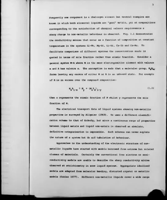
Frequently one component is a chalcogen element but several examples are

known in which both elemental liquids are 'good* metals, yet at compositions

corresponding to the satisfaction of chemical valence requirements a

sharp change to non-metallic behaviour is observed. Fig. 1.1 demonstrates

the conductivity minima that occur as a function of composition at constant

temperature in the systems Li-Pb, Mg-Bi, Li-Bi, Cs-Sb and Cs-Au. To

facilitate comparison of different systems the concentration scale is

quoted in terms of mole fraction rather than atomic fraction. Consider a

general system M-A where M is the more electropositive element with valence

m and A has valence a. The assumption is made that a molecular group, v w

forms leaving ¿my excess of either M or A in an unbound state. For example

if M is in excess over the compound composition:

M A, = M + (M A ) ,

x 1-x y a m 1-y ( 1 . 1)

then x represents the atomic fraction of M whilst y represents the mole

fraction of M.

The electrical transport data of liquid systems showing non-metallic

properties is surveyed by Allgaier (1969). He uses a different classifi­

cation scheme to that of Enderby, but since a continuous range of properties

between liquid metals and liquid non-metals is observed an absolute,

definitive categorisation is impossible. Such schemes can never explain

the nature of a system but do aid tabulation of behaviour.

Approaches to the understanding of the electronic structure of non-

metallic liquids have started with models borrowed from extreme but related

classes of materials. Certainly the conventional free electron or semi­

conductivity models are unable to describe the sharp conductivity minima

observed at stoichiometry in some liquid systems. Appropriate idealised

models are adapted from molecular bonding, distorted crystal or metallic

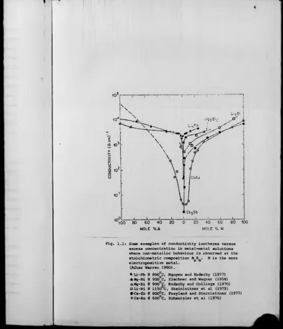
Fig. 1.1: Some examples of conductivity isotherms versus excess concentration in metal-metal solutions where non-metallic behaviour is observed at the stoichiometric composition M A . M is the more

ci ra electropositive metal.

(After Warren 1980).

• Li-Pb @ 800°C, Nguyen and Enderby (1977) AMg-Bi 0 900°C, Ilschner and Wagner (1958) AMg-Bi 0 900°C, Enderby and Collings (1970) □ Li-Bi 0 1150°C, Steinleitner et al (1975) ■Cs-Sb 0 800°C, Freyland and Steinleitner (1977)

of properties and clearly the model most suited to a given system is the

one which best emphasises its particular behaviour. For example, liquid

Mg^Bij i* relatively highly conducting and a metallic model is probably

closest, whilst molten selenium is best described by a molecular bond

model. One feature common to all models is the appearance of a dip in the

density of states curve near the Fermi Energy, E^,. Such a dip is known

as a pseudogap and can be thought of as corresponding to the crystalline

semiconductor band gap.

Interest in the electronic structure of non-mctallic binary liquids

has concentrated experimental research in thermoelectric measurements:

conductivity a , thermopower S, and Hall coefficient R . There is a relative rl

paucity of structural, magnetic and optical information which is in no

small way associated with the severe experimental difficulties associated

with the systems of interest. Low temperature approaches to electronic

structure such as electronic specific heat or do Haas van Alphen effect

measurements are clearly precluded. The high temperature and chemical

nature of many constituents often result in corrosive liquids with

appreciable vapour pressure, such that the choice of suitable containment

and electrode material requires much auxiliary effort.

This work investigates the composition dependent metal-nonmetal

transition in the systems Cs-Au and Cs-Sb, and the temperature dependent

metal-nonmetal transition in Se-Te. Each represents a different subgroup

of liquid binary alloys: liquid CsAu turns out to be a molten salt composed

of Cs+ and Au ions, the liquid semiconductor Cs^Sb is covalently bonded

with electronic conduction, and Se-Te is composed of a covalent extended

network. Such differences will be reflected ¿n the electronic structure,

but discussion of each system is deferred to the appropriate chapter where

a full description of the experimental and theoretical background is

6

For a metal non-metal transition which occurs as a function of

composition in a binary liquid alloy there are three regions of interest.

First of all at metal rich compositions the system is metallic and nearly

free electron concepts are appropriate. Secondly, the nature of the

transition from extended to localised states which often occurs near

y = 0.50 mole fraction excess metal is of considerable interest. It

seems unlikely that any one model can adequately explain the roles of

disorder, electron-electron correlation and the relative ionicity/

covalency of chemical bonding in the many different systems, thirdly,

what is the nature of the localised electron states when the stoichiometric

compound has a small excess of metal, and which physical and chemical

properties are essential to stabilise localised states in the liquid?

1.2. Bonding

Many binary liquid alloys exhibit anomalous properties at a characteristic

composition M_^A^ satisfying common chemical valence requirements. The

bonding of a compound is frequently expressed in terms of three extreme

models, although in reality the true picture must be intermediate.

1. Molecular or directed covalent bonds: the valence requirements

are satisfied within a molecule and the liquid consists of

electrically neutral molecules.

2. Ionic bonds: the s- and p- valence electrons are localised

on the electro-negative ion.

3. Mixed bonds: a fraction of s- and p- electrons are localised

with the remainder involved in an extended covalent network.

Covalent bonding is more familiar in light elements because their

intermolecular bonding is weaker and intramolecular stronger than for heavy

elements, (Phillips, 1973). Atomic orbitals of heavy elements are not as

mor«_

other than just those of the valence electrons play a role in bonding.

Covalent bonds in heavy element alloys are therefore less directional

ond con

readily acco«w«r*»dAt‘£. distortions which alter the bond angle. These

effects can be considered to add a partial metallic character to cova­

lent bonding in heavy metal alloys.

Since the electronic character of a material is intimately related

to the range of chemical interaction between the constituents a know­

ledge of bonding might be expected to allow the prediction of the nature

of the compound. Generally the greatest difficulty lies in deciding the

charge distribution per bonded atom, or the ionicity of the bond. An

empirical guide to ionicity is provided by the electronegativity difference

(Pauling, 1960)

AX = X. - X

A M (1.2)

Electronegativity, X, is a measure of the attraction of an element for a

valence electron and as such it is a real property of an element. However

it is inexactly defined and various authors dispute the best way of

determining electronegativity (Gordy and Thomas, 1956; Pauling, 1967;

Phillips, 1970). In particular the value for one element is not independent

of the second element in the bond. However the different electronegativity

values lead to similar predictions for values of AX. The bond ionicity,

I = P/ed, where P is the dipole moment of the bond and d the bond distance,

is related to AX by Paulings empirical relationship

1 = 1 - exp(-AX2/4) (1.3)

Howeyer the possibility of complex formation complicates the evaluation

of ionicity. The complexing ratio R is defined as the ratio of the co­

ordination number of an atom to its valence. Phillips (1973) gives the

effective ionicity Ic as

I -c

8

In a liquid, thermal disorder will prevent R having a value greater

than six.

At compositions away from stoichiometry the electronic structure

is strongly related to the nature of the bonding of the excess element.

Cutler (1977) suggests that the best guide is whether, or not the excess

element bonds covalently to itself, otherwise metallic bonding of the

excess is assumed. For instance in the system M-A if element A is Te

and is in excess it can covalently bond to itself, and this will happen

even if the M-A bond is ionic.

A further complication is that excess of an element of mixed valence

may bond with the mixed valence. For instance, Cu is found with equal

preference for its two options 1 and 2. For the case of In a valence of

3 tends to be preferred to 1.

1.3. Liquid Structure

Structural information about liquids is in principle most directly

obtained from neutron or X-ray diffraction studies (Enderby, 1974). The

quantity obtained from a diffraction experiment is the static structure

factor S(Q), but several experimental corrections are required to the

raw scattered intensity, see Enderby (1968) for neutrons, Pings (1968)

for X-rays. S(Q) is then related to the radial distribution function g(r)

by means of a Fourier transform

In practice truncation errors are introduced since the upper limit is

(S(Q)-l) Q2 dQ (1.5)

o

usually a, 12 8 and additionally the random error in S(Q) creates a

cummulative error at low r after the transform. North et al (1968)

g(r) describes the average atomic arrangement of the atoms in the liquid,

and is defined so that the average number density of atoms in a spherical

shell of radius r about any given atom is given by g(r) multiplied by the

average number density of the whole liquid.

In the case of binary liquid alloys M-A it is necessary to introduce

three structure factors S , , S , each of which has a corresponding

MM MA AA

pair distribution function g , g , g . Experimentally the total

co-MM MA AA

herent scattering intensity must be measured in the same alloy on three

separate occasions with different form factors. Two possible methods are;

neutron diffraction using isotopically enriched samples (Edwards et al,

1975), or X-ray diffraction of several concentrations relying on the

variation of form factor near the absorption edge (Waseda and Tamaki, 1975).

The "bench marking" technique of Enderby (1978) enables structural

studies to be i n t e r p r e t ^ in terms of the bonding near stoichiometry.

In this approach structural studies of liquids with reasonably well under­

stood bonding are used as a reference for the liquid alloy under investi­

gation. The reference categories

are:-1. symmetric ionic, NaCl

2. non symmetric ionic, BaCl2

3. incomplete ionic, CuCl

4. molecular, TiCl. 4

5. extended covalent network, Te.

To date there is little structural information on binary liquid

systems, but the ionic character of both CsAu and Li^Pb has prompted

the suggestion that all metal-metal systems are ionic to first order

(Enderby, 1978). Thi3 is not necessarily at variance with the experi­

mental observation of conductivities greater than expected for a molten

salt. For instance, both Li^Pb and Mg^Bij have o = 50 0 1 cm 1 just

10

contribution is present in addition to any ionic conduction in these

systems.

1.4. Metallic Conductors

The distinction between crystalline metals and insulators is based

on ideas proposed by Wilson (1931). At absolute zero metal is a material

in which one or more of the energy bands is partly occupied, whereas in

an insulator all bands are either completely full or empty and an energy

gap separates the occupied and vacant states. The distinction between

insulators and semiconductors is less clear and depends upon the magnitude

of the energy gap. When the gap is sufficiently small that significant

numbers of electrons can be thermally excited the material is termed a

semiconductor, whereas insulators have energy gaps of <, 3eV and negligible

carrier densities •

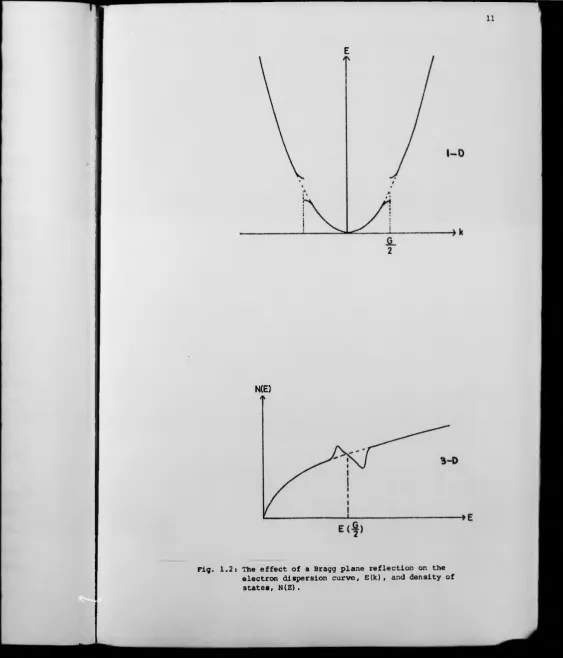
A solid crystal with a periodic lattice has an electronic structure

which can be described in momentum space on the basis of the nearly free

electron model. (Faber, 1972). The free electron parabolic dispersion

curve is modified by long range order which eliminates all the Fourier

components of the interaction potential except at K = 4G to create an

energy gap at the Bragg planes. Consequently the density of states shows

a small perturbation which can result in a net decrease in energy AE

| V ( G ) i f the Fermi energy, E^, lies in this region. Fig. 1.2.

In a liquid the atomic arrangement must be represented by an isotomic

probability distribution with the destruction of long range order. The

simplification of electron band structure results in a spherical Fermi

surface, but the electron-ion and electron-electron interactions remain

important. See for example the review by March (I960) on electronic

E

N(E)

12

For many liquid metals the nearly free electron theory of Faber

and Ziman (1965), (Faber, 1972) is well supported by experimental

investigations of electrical conductivity. These materials have values

path compared to interatomic distance, X > a. The weak scattering of

electron plane waves is treated by the Born approximation and the main

problem is the choice of an appropriate pseudopotential. The conductivity

may be expressed as

is found satisfactory in pure liq metals, but the situation is less

clear for alloys.

1.5. The Pseudogap in Non-Metallic Liquids

Cohen, Fritzche and Ovshinsky (1969) and Davis and Mott (1970)

discuss a general model for electron transport in amorphous semiconductors,

which was developed for the case of non-metal lie liquids by Mott (1971),

and is generally referred to as the pseudogap model.

In the study of impurity conduction in crystalline semiconductors

it is well known that potential fluctuations at sites of impurity atoms

cause the normal band edges to show a smearing or 'band tailing'.

(Halperin and Lax, 1966, 1967). If short range order characteristic of

covalent bonding exists then the introduction of long range disorder as

in amorphous or liquid systems does not necessarily destroy the band gap

of a crystalline semiconductor. Instead it results in the smoothing of of a typical of solid metals (0 £ 3000 ft 1 cm X) and a long mean free

(1.6)

where is the Fermi surface area.

The thermopower S is related to o through

2 2

ir k T dlno

(1.7)

3 e dE

E=E, F

and the elementary equation for the Hall coefficient 1 nec

Van Hove singularities and a spreading of the density of states into

the gap to produce a pseudogap, Fig. 1.3a. This approach; adding dis­

order to a band structure in which a gap already exists; is known as

the distorted crystal model and has been treated theoretically by

Gubanov (1965) with emphasis on the amorphous state.

In the metallic approach to the pseudogap model the starting point

is the NFE density of states. With the introduction of stronger electron

ion interaction and long range disorder the electron mean free path, X,

decreases and the Born approximation is no longer valid. A large dip

may develop in N(E) associated with a particular geometric cluster of

atoms, stabilised by a structure sensitive decrease in energy if E is r

near the minimum, Fig. 1.3b. In this picture thermal disruption of

clusters would lead to an increase of the density of states washing out

the pseudogap. With X 'v a, where a is the interatomic spacing, Mott

(1967) argues that the change in the density of states at the Fermi

level becomes the controlling factor for o, and

22 o = 1 e ,

3ha (1.9)

where

N(Ep )

N(Ef ) (1.10)

Free electron

This approach is expected to be valid for 150 < a < 3000 fi 1 cm 1 which

is called the diffusive regime. Evidence in support of the diffusive

mechanism of transport is provided by magnetic measurements where the

data fits the predicted equation. E.g. nuclear magnetic resonance shift

ij

a a (Warren, 1972a), (Seymour and Brown, 1973). The expression for

thermopower is also satisfactory,

d In N(E)

2

,

2

_

s-V —2

but there are problems associated with momentum transfer in the expression

for the Hall coefficient. Friedman's theory (1971) accounts only partially

for the experimental behaviour.

C.g-1 (1.12)

Free electron

The Mott g factor introduced in describing diffusive transport is occasion­

ally troublesome because of the difficulty of knowing just which electrons

to count in the free electron approximation. For lower values of a the

spatial character of the electron states acquires great significance.

In a tight binding formulation weakly overlapping atomic states form

extended states in a band of width T = 2Jz where J is the overlap integral

and z is the coordination number. Anderson (1958) showed that in the

presence of potential fluctuations AV, localised states occur when

AV > nr, where n is some critical value, later evaluated by Mott (1972a)

to equal 2. Mott (1968) developed Anderson's theory to consider whether

localised and extended states are separated in energy within a band. For

a large enough N(E) there will be available sites sufficiently close in

energy for an electron to diffuse throughout the volume. For a given AV

there is a critical density of states below which the tunnelling distance

is too large and the electron becomes localised in a given region. Mott

suggests that the transition occurs for g “ 1/3.

It is noteworthy that there is still some dispute as to whether

localised states do form as a result of potential fluctuations, (see

E.g. Thouless, 1972), but the concensus view is affirmative. Mott (1969)

has further suggested that the directional nature of non-s- electrons means

they are more likely to become localised than are s-electrons, since they

16

Hence there is a value of energy, E ^ , which separates localised and

extended states and a lower limit for non-activated conductivity must

exist. E is referred to as the mobility edge, since at finite temperatures c

the electrical conductivity of localised states is several orders of

magnitude smaller than that of extended states. Fig. 1.4. Motts equation

(1972a) for the conductivity due to extended states at the mobility edge

is

0(E ) c

0.025 e" ha

610 Q-1

a* (1.13)

where a * (8) is the interatomic distance (typically 48) and the coordination

number z = 6. This suggests the minimum metallic conductivity, o(E^) ^

150 fi 1 cm 1 , is the non-zero lower limit of conductivity in extended

states before a discontinuous transition to essentially zero electronic

conductivity in localised states occurs. The validity of the minimum

metallic conductivity concept is the subject of considerable current

interest. As a consequence of the exclusion of the electron wave function

from regions of potential fluctuations, Eggarter and Cohen (1970) and

Economou et al (1974) have proposed that a(E) decreases more rapidly than

2

N (E) and thus goes continuously to zero as E + E from above. It seems c

likely however that the disputed differences in the shape of o(E) near

are unimportant for liquids because they occur on a scale S kT.

If the density of states at the Fermi Energy, N(E ), is sufficiently

below the free electron value then the observed low conductivity due to

localised states is described by the empirical expression (Stuke, 1969)

AE

c = a (E^) exp(- A t) (1.14)

In principle for localised states below the mobility edge two conduction

processes are possible.

1. when 1 < o < 150 il ^ cm the predominant mechanism is the excitation

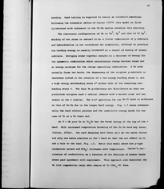
bonding. Band tailing is expected to create an interband pseudogap.

Following the extensive review of Cutler (1977) this model is first

illustrated with reference to the Tl-Te system assuming zero ionicity.

2 4 1

The electronic configuration of Te is 5s , 5p and that of T1 6p .

Bonding of two atoms is assumed to be a linear combination of p orbitals

and hybridisation is not considered for simplicity, although in practice

the bonding energy is usually increased as a result of mixing of atomic

orbitals. Bringing atoms together results in a decrease of energy for

the symmetric combination which concentrates charge between atoms and

an energy increase for the charge cancelling combination. A Te atom

normally forms two bonds; the degeneracy of the original p-orbitals is

therefore lifted in the creation of a low energy bonding state o, and

a high energy antibonding state a* either side of the remaining non­

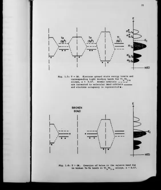
bonding state it. The four Te p-electrons are distributed so that one

p-electron occupies each c orbital (shared with a bonded atom) and two

remain in the tt orbital. The a - a * splitting for the Te-Tl bond is different

to that of Te-Te due to the larger bond energy. Fig. 1.5 shows schemati­

cally the bond orbital process and the associated energy bands for the

case of T1 at a Te chain end.

At T = OK pure Te or Tl^Te has the Fermi energy at the top of the tt

band. With increased temperature breaking of the Te-Te bond may occur,

(Cutler, 1971a). For each dangling bond there will be two extra states

and only one extra electron in the it band so that the net effect is to

add a hole to the band. Fig. 1.6. Hence this model shows how p-type

conduction arises and N(EF ) increases with temperature. Cutler's cal­

culation of conductivity as a function of the fraction of broken bonds

shows good agreement with experiment. This approach also describes the

?0

E

N(E)

Fig. 1.5: T = OK. Electron ground state energy levels and corresponding tight binding bands for Tl^Te ^ alloys, x < 0.67. Atomic orbitals ---are converted to molecular bond orbitals.... — and electron occupancy is represented •.

E

BROKEN

BOND

N(E)

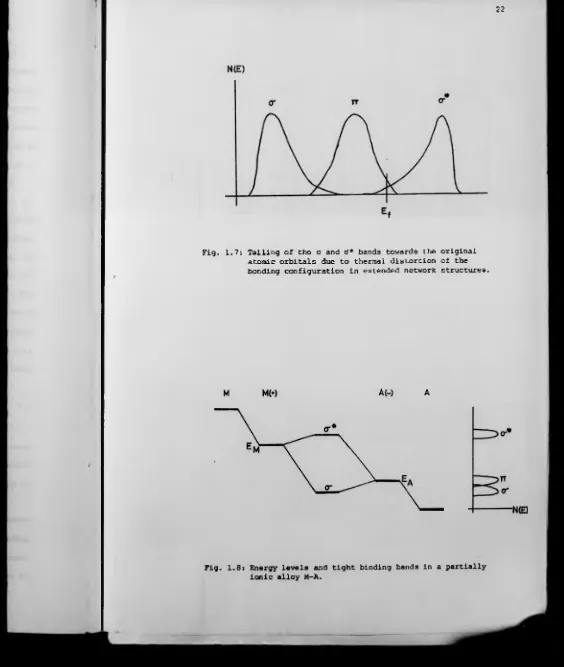
Another possible effect of non-zero temperature is a thermal

distortion of the bonding configuration. This would have the effect

of reversing the level splitting and result in a shift of discrete

states toward their original atomic orbital values. Thermal vibrations

would therefore cause the o and o* bands to have tails toward the it band

as shown in Fig. 1.7. Cutler (1971 (a)) claims that this process may

be more important than bond breaking in extended network structures.

A modification to the above molecular bond scheme is necessary in

the case of an alloy in which the constitutents have an electronegativity

difference such that ionicity might be expected to play a role. For

different atoms the initial atomic energy levels will be different,

but charge transfer shifts the levels toward each other, (see for example

Coulson, 1961). Fig. 1.8 shows schematically the result of charging

and of the subsequent a - a* splitting due to bonding. If A is taken

to be an element with some non-bonding states such as Te, the tight

binding o and it bonds are likely to overlap strongly as shown. If A

is a group V element then there is no it band since all three p-electrons

benefit energetically from forming a bonding orbitals.

1.7. Electronic Structure Away from Stoichiometry

There is a concensus view that a pseudogap exists in the density of

states at the stoichiometric composition of some liquid alloys systems.

However for compositions away from stoichiometry there is a wide diversity

of opinions.

Based on a model of Enderby (1973), the model of Roth (1975) has

however gained general acceptance for interpretation of ionic binary

systems. The electronic structure of a system M-A as a function of

composition is presented in Fig. 1.9. Band tails and possible regions

22

N(E)

Fig. 1.7: Tailing of the a and 0* bands towards the original atomic orbitals due to thermal distortion of the bonding configuration in extended network structures.

M

MW

A(—)

A

24

of A to M, the bonding electrons form a new band below the Fermi energy

which may or may not be separated from the conduction band by a gap. As

the concentration of A is increased the A band grows and E^, moves down

the conduction band since each A atom adds more states than electrons.

At stoichiometry E^ is located midway in the pseduogap. Excess of A

causes E to enter the valence band, which becomes a partly filled band F

of pure A in the limit of negligible concentration of M. The liquid

system Mg-Bi is thought to obey this model.

Cutler (1977) describes a modification of Roth's model for the

situation of partial covalent bonding between element M and a chalcogen,

A. Fig. 1.10 presents the main features. In M rich alloys the only

difference from the ionic case is the splitting of the valence band into

o and it states. Near stoichiometry the reduced M band has become an

impurity band which may be absorbed into the a* band. At stoichiometry

Ep is midway in the pseudogap. If excess A remains unbonded, then Ep

moves down the valence band as in the ionic model above. If A atoms bond

covalently to each other, then the valence band remains filled and insulator

behaviour occurs (at T = OK) as indicated in Fig. 1.10.

An alternative approach is provided by Enderby and co-workers (Enderby

and Simmons, 1969; Enderby and Collings, 1970), who speculate that the

Hall coefficient is a useful measure of the charge carrier nature and that

bound states due to molecular groups at stoichiometry form a band separated

in energy below the conduction band. E always remains in the conduction

band. A peak in R^ at stoichiometry therefore arises from depletion of

the number of free electrons arising from either excess M or A. A virtual

bound state near was suggested to explain the sign change of thermopower

at stoichiometry and the major criticism of this approach is the rather

Faber's (1972) model overcomes the thcrmopower difficulty by

assuming the excess element forms an impurity band near the bottom edge

of the conduction band, and therefore the N(E) has a different character

according to which element is in excess. The impurity band grows into a

fully-fledged band in the limit of excess concentration = 1. Although

qualitatively satisfactory a separate impurity band is unlikely unless

the Eg is large (and a small). Also impurity band conduction near

stoichiometry suggests N(E) would be very sensitive to composition,

but Cutler has shown that rigid bands are satisfactory in Tl-Te.

Several authors have approached the electrical properties of non-

metallic liquids through non-homogeneous structural models. (Hodgkinson

1971, 1973; Cohen and Jortner, 1973, 1974a; Bhatia and Thornton, 1970;

Cutler, 1976c). Density or concentration fluctuations within a sample

are considered to create well defined regions and conduction is deter­

mined by percolation processes. However thermodynamic considerations do

not lend support to this approach (see for example Cutler, 1977).

SI.8: The Effects of Correlation

The disorder-induced Anderson transition and the transition with

change of density in divalent metals are both examples of metal-nonmetal

transitions permitted in the approximation of non interacting electrons.

However the metal-nonmetal transition occuring for example in expanded

liquid alkali metals is inexplicable within the classical band model of

non interacting electrons. In many systems, if not all involving

localised states, electron-electron interactions (correlation) plays an

essential role as discussed with different emphasis in the work of Mott

26

For a crystalline array of one electron atoms at the absolute zero

of temperature Mott (1949, 1961) has shown that a sharp metal-nonmetal

transition occurs as the lattice parameter is varied. Defining the

number density of electrons as n, and a critical value as n^, then for

insufficient and the free electron gas crystallises into an insulating

state. A small number of free carriers is impossible since bound pairs

form (Mott and Davis, 1971), and hence a discontinuous change in the

number of carriers is predicted. Mott's criterion for the transition

is

where a* = effective hydrogen-like radius. H

Edwards and Sieako (1978) have shown the applicability of this equation

for a variety of materials over a range of nc equal to lO orders of

magnitude.

The role of the interatomic Coulomb energy was considered formally

by Hubbard (1964), who showed that a metal-nonmetal transition was

predicted without the need for interatomic Coulomb forces. The Hubbard

energy U is defined as the electrostatic repulsive energy of two electrons

located on the same atomic site, and for large interatomic separation

where r ^ is the electronic separation

Ej. is the ionisation energy

Eft is the electron affinity.

The Hubbard model predicts the splitting of a half filled conduction band n > n the ion potential is well screened and a metallic state is formed.

However for n < nc the screening of the long range Coulomb force is

a* = 0.26

H (1.17)

n c

2

U = <• (1.18)

r 12

occurs when U is approximately equal to the undistorted bandwidth and

the lattice parameter is such that the bands separate. At absolute zero

the lower band is full and the upper band empty. In the absence of long

range Coulomb forces no discontinuous change in the charge density is

expected.

The influence of correlation on metal-nonmetal transitions is

28

CHAPTER TOO

NUCLEAR MAGNETIC RESONANCE

2.1. Magnetic Susceptibility

Hie magnetic susceptibility x» is the most basic magnetic property

and may be expressed per mole, per unit mass or per unit volume. For the

interpretation of microscopic properties Xmo^e is the most useful and may

for instance be obtained from a combination of density data with x^j • X.fy10,s \&

determined by the Gouy Method. Nachtrieb (1962) and Gardner and Cutler

(1976) provide examples of the experimental approach necessary for the

high temperature study of liquids of interest in this work.

The total measured susceptibility is made up of principally two

parts: one due to the ion cores and the other to the conduction electrons

xtotal ~ Xion + Xcond (2.1)

core elec.

The diamagnetic susceptibility of the ion cores is often dominant so that

even in liquid metals the net effect may be diamagnetic or only weakly

paramagnetic (Dupree and Seymour, 1972). Estimates of the value of Xion

core have been made by direct measurements of ionic salts or by calculation

from the free ion wave function, but are not entirely satisfactory. This

uncertainty hinders the extraction of Xcon(j which contains information

about the electronic structure. The electrBnic susceptibility itself

contains both spin paramagnetism and orbital diamagnetism, and on the free

electron model its value is dependent upon the density of states at the

Fermi level, N(E ). However for real metals, electron-electron correlations F

lead to an enhancement of the static susceptibility (Pines, 1955) producing

Two cases are of special importance: for nearly free electron metallic

liquids a Pauli paramagnetism is expected.

(2.2)

P 2

X , = y u N (E )

*elec o B F

where y is the Bohr magneton. B

For a dilute concentration of localised electrons as found with excess

metal in a non-metallic compound or broken covalent bonds a Curie-type

susceptibility is appropriate.

elec

NV

3kT (2.3)

where y is the magnetic moment,

k Boltzmann constant,

T the absolute temperature

2.2. Introduction to Nuclear Magnetic Resonance

Nuclear magnetic resonance (NMR) is the spectroscopy of the nuclear

Zeeman energy levels in a static magnetic field, and was first observed

by Bloch et al (1946) and independently by Purcell et al (1946). An ex­

tensive literature has subsequently arisen on the many different aspects

and applications of NMR and therefore this chapter introduces only the

material most relevant to this work. A full discussion of the theory of

NMR is to be found in Abragam (1961) and Slichter (1978). The use of

pulses of power at a discrete frequency in the observation of NMR was

first put into practice by Hahn (1950). Hie behaviour of the spin system

is studied after the pulse is turned off, and the same spectral information

is obtained as in continuous wave experiments, with the added advantage of

direct access to spin relaxation information.

30

magnetic moment p and spin angular momentum fil_. These quantities are

related by the magnetogyric ratio y according to

Ihe interaction of the magnetic moment with an applied magnetic field B

is given by the Hamiltonian

where m is an eigenvalue of 1^, the component of Jt along which is

conventionally taken to define the z axis. Transitions can be induced

by supplying radiation tuned to the energy difference between neighbouring

levels, and thus the resonance condition is given by

Classically the resonance frequency corresponds to the Larmor frequency

of gyroscopic precession of a magnetic moment in the applied magnetic field.

Strictly the time varying field is a rotating field and the direction of

notation must be included

For nuclear spins u corresponds to radio frequencies.

Occupation of the energy levels is described by a Boltzmann distri­

bution when the nuclear spins are in thermal equilibrium with their

environment, the "lattice". Despite the equal probability for stimulated

upward and downward transitions a net absorption of energy therefore occurs

because of the larger number of lower energy spins. To prevent saturation

there must be some means of restoring thermal equilibrium when the levels

become equally populated, and this is provided by a relaxation interaction

P. “ yfii (2.4)

(2.5)

and this results in the equally spaced Zeeman energies

E = - YfiB m

m o (2.6)

ai = yB

o (2.7)

between the spins and the lattice.

Consider a system of N identical nuclei of spin I = *j in a static

magnetic field Bq creating Zeeman levels separated by 2pbQ . Let N^,

be the occupancy of the lower and upper levels respectively. In thermal

equilibrium N N 2 1 (2.9)

If the level occupancy is disturbed by an r.f. field then the return to

thermal equilibrium when the r.f. field is switched off is characterised

by

dn dt

- (n-n ) o

(2.10)

where N^-N2 at thermal equilibrium

instantaneous population difference

(W+ + W+) = the sum of the probabilities per second for

spin lattice transitions up and down.

is therefore a characteristic time associated with the approach to

thermal equilibrium and is related to the microscopic details of the spins

and the lattice. The study of T^ provides much information concerning

the dynamic nature of the nuclear environment.

Spin-spin couplings allow the establishment of thermal equilibrium

among the spins. Such processes vary the relative energies of the spin

levels and are characterised by a relaxation time T^.

The non-zero 'natural' width and shape of a resonance absorption line

arise from a combination of the finite lifetime (T^ process) and energy

level fluctuations (T2 process). The line shape function for Lorentz

lines common in liquids is

g(u>)

2 2

l+T0 (u-m )

z o

32

where the half width at half height is given by

Au. = (2.12)

S T2

The observed experimental linewidth V t* may have an additional contribu­

tion due to magnetic field inhomogeneity, which causes spins in different

parts of the sample to precess at slightly different frequencies.

-i- = — + — (2.13)

T* T 2 T 2

natural magnet

The effect of motion in a non-viscous liquid is to reduce all

couplings with the nuclear spin, such that the .c.f".S. local field

is much less than in the rigid lattice. The dominant contribution to the

linewidth is therefore due to lifetime broadening and in the limit of

extreme motional narrowing, wx << 1, increases until T 2 = T^. For

viscous liquids in which > T2 a long correlation time x is indicated,

and the T ^ / ^ ratio enables x to be determined. A generalised form of

the T 1 and dependence on x, valid for any interaction, is presented

in Fig. 2.1. (see for example Slichter, 1978) .

In condensed matter there is an ensemble of spins and for each the

actual field experienced is modified from Bq by an average internal field

associated with the nuclear environment. The resonance condition can thus

be written

W = Y (B + AB) (2.14)

o

and measurement of the nuclear resonance shift provides information about

the static aspects of interactions with the nuclear spin. These will

generally include nuclear dipole-dipole interactions, magnetic couping

of electrons to nuclei, and the strong electrostatic effects between

RELAXATION

TIME

34

An important consideration for NMR in metals is the exclusion of

r.f. magnetic fields by the r.f. skin effect, described by

6 = (2.15)

where 6 is the skin depth

a is the electrical conductivity

V is the magnetic permeability.

Frequently metallic samples are divided into particles smaller than the

calculated skin depth, but it is sometimes convenient to work with bulk

samples. When the skin depth is less than the particle size the nuclear

resonance is confined to only nuclei near the surface and a reduction of

signal size results. The shape of the resonance line is also distorted

due to the interaction of nuclear spins with the induced eddy currents.

A further problem is the reduction of the Q factor of the r.f. coil caused

by such a lossy sample which also reduces the signal to noise ratio.

2.3. Resonance Shifts and Relaxation Data

A classical description of the net magnetisation during a pulsed

nuclear magnetic resonance is now presented. The validity of a classically

precessing magnetisation in a quantum mechanical system possessing only

(21 + 1) states along is explained by the fact that the expectation

value of p_ has an exactly similar time dependence to that of the magnetisa­

tion vector M (see for example Slichter, 1978) .

A static magnetic field produces a preferred orientation of the

nuclear spins and a net magnetisation M along the z axis. An additional

B^ rotating in the x-y plane at frequency w causes M to precess about the

direction of the effective field. It is convenient to pursue the description

the laboratory 2 axis but the x ^ y 1 plane rotates at u>. (Rabi et al,

1954). In the rotating frame the spin behaves as though subjected to

an effective field given by

B = B + = + B

=eff —o Y — 1 (2.16)

Hence for the 'on-resonance' situation of B^ rotating in the laboratory

frame at the Larmor frequency id^, the effective field is in the direction

of B ^ . Assuming B^ to be directed along the x1 axis then the magnetisa­

tion rotates in the y^-z^ plane of the rotating frame as shown in Fig.

2.2. In a time t the angle 6 through which M precesses is given by

6 - YBjtj,

Two pulse lengths are particularly important:

,0

(2.17)

The 90 pulse, tn , which causes M to tip into the x y plane and1 1

point along the y axis.

2 " YV n

(2.18)

2. The 180 pulse, which causes a precession of M until it loO

points in the -z direction.

ïï

YB1T180 (2.19)

The generation of a component of magnetisation in the x -y plane

induces a voltage at frequency u)q in a receiver coil placed in the plane

and so enables resonance to be detected.

In the simplest theory, pulses are assumed to be so short that no spin

relaxation processes occur during the pulse. Following the end of the pulse

the interaction of the spins with each other and the lattice causes the

magnetisation to return to its equilibrium value The relaxation of

the component is characterised by the spin-lattice or longitudinal

spin-Fig. 2.2s On resonance rotation of the magnetisation vector in the rotating frame of reference. The B^ field is applied along the x ' axis and precession occurs in the z '- y ' plane. In a time tp, the angle swept out, 0 = YB, t .

spin or transverse relaxation rate R2 = /T2 . The decaV to zero of the

initial signal amplitude created by H i i is due to spin dephasing and x y

is known as the free induction decay (F.I.D.). For a sample not in a

perfectly uniform magnetic field such dephasing is increased and the

signal decays with the characteristic time T* .

For the 'off resonance* situation of the r.f. at a slightly different

frequency to the Larmor value, M rotates relative to the rotating frame,

and the F.I.D. shows wiggles within the decay envelope at a beat frequency

corresponding to the difference from resonance frequency.

The measurement of the F.I.D. following a 90° pulse is the basic way

of determining spectral information. The position of the resonance may

be obtained by noting both the frequency of operation and the beat fre­

quency evident in the F.I.D. wiggles. Repeating this procedure at a

different operating frequency yields a unique value for the resonance

frequency. Nuclear magnetic resonance shifts are then determined by

taking as reference the resonant frequency of the same nucleus at infinite

dilution in a suitable solution at the same field, or equivalently the

resonant field of the reference at the same frequency.

Alternatively, the resonance lineshape can be obtained using pulsed

NMR as pointed out by Clark (1964). This relies on the fact that the

steady state unsaturated absorption x" is proportional to the Fourier

cosine transform of the F.I.D. envelope and the disperison x' is pro­

portional to the Fourier sine transform. (Lowe and Norberg, 1957). By

sweeping either frequency or field the output of a boxcar integrator

sweeps out the resonance lineshape as discussed further in chapter 3.

Calibration of the sweep thus enables the resonance position to be obtained.

It is generally necessary to distinguish three relaxation times

characterising nuclear magnetic resonance:

T * S T S T

In solids and viscous liquids the correlation time for nuclear

interaction is long enough to distinguish T2 < T^. The determination

focussing of the spins then occurs at time 2t along the -y axis to

create the so-called echo. A series of echo amplitude measurements as

a function of 2t allows the determination of 'F^.

The simple spin-echo technique is limited in applicability because of

molecular diffusion which reduces the echo amplitude by a term dependent

upon magnetic field gradients G, and the diffusion coefficient D. (Carr

and Purcell, 1954).

The strong T dependence has most influence on measurements of long

but must be borne in mind in situations where T* is artifically reduced

in order to make the echo visually sharper. Problems are indicated when

the echo amplitude is seen to decrease faster than exponentially.

2.4. Nuclear Resonance Shifts

In a fixed magnetic field nuclear magnetic resonance in metals

generally occurs at a higher frequency than for the same nucleus in a

diamagnetic sample. Equivalently at a fixed frequency the static field

required for resonance is lower in a metal. The fractional shift is

called the Knight shift, K (Knight, 1949).

by the use of Hahn's (1950) 90°-r-180° spin echo sequence. Following

the 90° pulse the spins in the x1y1 plane are allowed to dephase for a

period T before a 180° pulse causes precession about the x^ axis.

Re-1

A2t a exp -2 x (2.2 2)

40

Au _ AB _(2.24)

B is the resonance field in the metal. m

K is typically <v< 1% and is independent of the value chosen for wd (or

B ). A paramagnetic shift is taken to be positive, m

In metals the dominant contribution to the local magnetic field

at the nuclear site, AB, arises from the magnetic contact hyperfine

interaction which couples nuclear and electronic magnetic moments

where A is the hyperfine coupling constant

6(r) is a delta function.

S-type conduction electrons have a net polarisation due to the external

site they produce an extra magnetic field proportional to Bq . The Knight

shift can be expressed as (Townes et al, 1950)

n is the number density of electrons.

In principle equation (2.26) can be used to obtain the density of

H = AI.SÓ(r) (2.25)

field Bq , and because of their finite probability density at the nuclear

m 2

3 <I*(0)|2>f ft x! p

■v (2.26a)

(2.26b)

*2

2

where <|t|i(0)| >„ is the electronic probability amplitude at the nucleus F

averaged over states at the Fermi level

ft is the electron normalisation volume

F

* is the Pauli paramagnetic susceptibility per unit volume.

p

problems arise due to the difficulty of determining <|tMO)| > . Electron 2

spin resonance experiments can yield this factor directly, but this has

only been achieved for alkali metals, (Schumacher and Slichter, 1956;

can be used together with some estimate of the penetration factor, £.

£ is typically 'v- 0.5 (Knight, 1956), and therefore tends to cancel the

further problem of the electron-electron susceptibility enhancement,

leading to agreement with calculated values of K within about + 30%.

The nuclear resonance shift is a measure of the contact interaction

but this cannot generally be obtained unambiguously due to the presence

of other contributions to the observed shift. For instance, polarisation

of the s-electron in the core by the conduction electrons creates an

additional resonance shift, S , called the core polarisation shift. cp

This is difficult to evaluate since the effect of s, p and d fractional

character of the conduction electrons on each core state has to be individu­

ally determined. Some contributions may be negative producing a reduction

in the observed shift, but S is unlikely to be greater than + 15% of K.

cp

-The nuclear resonance shift, S , due to the orbital motion of the

conduction electrons is approximately described by Noer and Knight (1964)

where XQ is the orbital susceptibility

r is the mean electron orbit radius.

Except for transition metal nuclei Sq is small compared to K and will be

neglected.

2

Ryter, 1960). Values of 1^(0) | from atomic optical hyperfine structure

(2.27)

o

(2.28)

observed resonance position of a given nucleus, creating further

difficulties in the extraction of the conduction electron contribution

to the observed shift. The shifts in insulators are known as chemical

shifts and arise from the orbital motion of bonding electrons (Ramsey,

1950). This changes the charge distribution around an atom and mixes

high states into the ground state. A diamagnetic shift is defined to

be positive.

S

-2vi e 2i 2z o_____

3mAE

<

7

>

where z is the number of valence electrons

¿iE is the energy difference between ground and excited state.

Chemical shifts are generally at least an order of magnitude smaller

than Knight shifts and are dependent upon the molecular environment,

(being anisotropic in solid compounds). A chemical shift can in prin­

ciple be related to electronegativity since a purely ionic closed shell

configuration will create no shift.

Finally, localised paramagnetic centres in an insulating system

create a shift due to the hyperfine contact interaction which is

characterised by a Curie susceptibility

Ab Po .ye S(S+1) — = — czA-

---B 2ir yn 3kT (2.30)

where A is the contact hyperfine coupling constant with a centre of

spin S

c is the concentration of paramagnetic centres

z is the co-ordination number of a paramagnetic centre

For this work, a salient feature of this shift is the linear dependence

■*-/3 on concentration which should be contrasted with the (number density)

42

dependence of shift in a metallic system. Furthermore, both expressions

is proportional to the electronic susceptibility through a constant

term involving the coupling constant A. An estimate of A is therefore

obtained from the gradient of a shift versus susceptibility graph, and

this may aid interpretation of relaxation data as discussed in §2.5.

2.5. Spin Lattice Relaxation

-tran S W S * co«*for»er&r of* On a semiclassical picture any time dependentj^nuclear spin-lattice

interaction with a non zero Fourier component at the resonance frequency

u) will induce transitions and allow the spin to relax. (Bloembergen et o

al, 1948). Quite generally the spin-lattice relaxation rate, R ^ , can

be written

R^ = (interaction s t r e n g t h ) ^ (2.31)

and various approaches to express R^ in terms of the lattice parameters

are discussed by Abragam (1961).

The concept of a spin temperature can be used in the case where

spin-spin coupling is much stronger than the coupling of the spin to

the lattice. The strong interaction establishes a common temperature

for the spins which is then changed by interaction with the lattice. How­

ever, in the case of motionally narrowed resonances the density matrix

formalism is most appropriate. Here the lattice parameters are taken

to be random functions of time and are described by their probability

distribution using the density matrix, p: a quantum operator which

performs the role of the classical density of points in phase space.

This approach is exactly equivalent to time dependent perturbation theory

but provides a more convenient way of computing thermal equilibrium

properties of a system (Slichter, 1978).