A Simple Statistical Estimation of One’s Performance in an MCQ Examination, Based Upon Mock Test Results, Using Binomial Distribution of Probability

http://dx.doi.org/10.4236/ojs.2012.24057 Published Online October 2012 (http://www.SciRP.org/journal/ojs)

A Simple Statistical Estimation of One’s Performance in an

MCQ Examination, Based upon Mock Test Results, Using

Binomial Distribution of Probability

Sudipto Roy1, Priyadarshi Majumdar2* 1

Department of Physics, St. Xavier’s College, Kolkata, India 2

Jyotinagar Bidyasree Niketan Higher Secondary School, Kolkata, India Email: [email protected], *[email protected]

Received June 4,2012; revised July 8, 2012; accepted July 20, 2012

ABSTRACT

A simple statistical model is proposed regarding the estimation of one’s overall performance in an MCQ examination along with the calculation of probability of obtaining a certain percentage of marks in the same. Using the data obtained from the results of a sufficiently large number of mock examinations, conducted prior to the main examination, certain parameters quantifying one’s knowledge or preparation for the examination has been calculated. Based on those pa- rameters, the probability of obtaining a certain percentage of marks has been computed using the theory of binomial probability distribution. The dependence of this probability function on various parameters has been depicted graphi- cally. A parameter, called the performance index, has been defined in terms of the expectation value and standard de- viation of marks computed from probability distribution. Using this parameter, a new parameter called the relative per- formance index has been defined. This index estimates one’s performance with respect to the best possible performance. The variation of relative performance index with respect to the preparation index has been shown graphically for dif- ferent parameter values quantifying various aspects regarding the examination and the examinee.

Keywords: MCQ; Preparation Index; Knowledge Index; Application Index; Performance Index; Relative Performance; Binomial Probability Distribution; Estimation of Examination Result

1. Introduction

Although it is widely acknowledged that the scores or grades one makes in an examination can never be the ultimate judge of a student’s talent or academic capabil- ity. But for all practical purposes the importance of an examination is universally accepted. It is a possible method to assess students because it judges them by a common technique (having the same set of questions) applied to all the examinees under the same circum- stances (at least tried to be maintained). The general ex- amination process, with long or descriptive answer type questions, has a major disadvantage that there exists no unique answer to a particular question, for any discipline whatsoever. In other words, it is impossible to prepare a unique model answer for a descriptive type question pa- per. Therefore, we have an obvious lack of uniformity in the ways of manual evaluation of the answer scripts by different examiners. It is not possible to use computers to evaluate such answer scripts because of the absence of a unique set of model answers. In-depth knowledge of sub-

ject and critical analysis are required to examine such scripts. An examiner, well versed with the subject, can only do this properly. Other shortcomings of the old ex- amination process are that its implementation has a lot of difficulties and it is very much time consuming because of its manual nature of evaluation. Despite all these dis- advantages the old examination process is still of great importance worldwide for University degrees that we are very much concerned about.

correct option). The degree of difficulty or stiffness of the question paper becomes higher as the given options become closer to one another in meaning. A great ad- vantage with this MCQ type examination is that one can maintain uniformity of questions and evaluation process because of the availability of unique model answer. Apart from this, computers can be programmed to evalu- ate such answer scripts, reducing the cost and time of the process. The shortcomings of MCQ are that an examinee can make high scores in this kind of tests without having in-depth knowledge of the subject. Taking recourse to wild guess one can score moderately high marks without having any workable knowledge in the subject.

Srinivasa and Adkoll [1] studied the application of MCQ in medical education and suggested the necessity of developing a MCQ bank for future purpose. In another particular study [2] the three option and four option MCQ tests in nursing education are compared with each other and it was concluded that the three option tests performs equally well in compared to the other. The ad- ditional option(s) most often does not improve the test reliability and validity. Costa, Olivera and Ferrao [3] studied the psychometric properties of the three multiple choice tests used to measure skills in Statistics in the scope of the engineering and management courses of the University of Minho. Steif and Dantzler [4] quantified the learning of concepts in Statics using MCQ. Steif and Handsen [5] analysed the results of MCQ tests that has been uses to measure learning in statics. In a more recent work Ventouas et al. [6] on the other hand discussed about the relative advantage and disadvantages of MCQ and CRQ (constructed response) based papers. In fact they admitted the advantages of MCQ with positive and negative marking concerning the objectivity in the grad- ing process and speed of production of results.

MCQ s has a long and widespread history of use in support of teaching and assessment across a range of disciplines as mentioned. The increased use in the recent years relates to the governance and resource of higher education and changing student characteristics [7]. There is a substantial amount of assessment literature associ- ated with MCQ s and it supports claims of benefits aris- ing from effective practice and also identifies significant limitations when application is inappropriate or the need for assessment efficiencies takes precedence over peda- gogical concerns and considerations [7-11]. MCQs have proved effective ways of assessing learning at the lower levels of Bloom’s Taxonomy [12], identification and understanding. However, MCQ s can be constructed to be more challenging than was once believed [13] and so application at higher levels of Bloom’s Taxonomy has also been demonstrated [14].

In contrary one of the most frequent criticisms of MCQ s is that they trivialize the learning process through

an over emphasis lower levels of cognitive demand [15] and that this often fails to reflect the true intentions of course learning objectives. According to Paxton [16] the learners may be quite skilled on taking MCQ tests but their ability to solve problems, exercise personal judg- ments and to communicate their understandings may remain underdeveloped. Other research [17,18] has found that students perceive MCQ s as assessing at a surface level and this consequently misdirects and other- wise influences the way in which they prepare for ex- aminations.

In order to overcome such difficulties, the questions are chosen uniformly from all parts of the syllabus. These are of different patterns, such as knowledge based, understanding based, application based and skill based in appropriate proportions. The answers given at the end of each question must appear to be very close to one an- other to curb the tendency of answering without knowl- edge of the subject as mentioned earlier. We generally have negative markings for wrong attempts in MCQ examinations to discourage the random guessing process to a large extent.

In a recent work Ding and Beichner [19] discussed about some commonly used approaches of MCQ data analysis in physics research namely, classical test theory, factor analysis, cluster analysis, item response theory and model analysis.

2. Modelling

In the present article a statistical model has been devel- oped regarding the estimation of probable performance of a student taking a MCQ examination. Some parame- ters, quantifying ones knowledge and understanding of the subject, have been defined in this context. Using this model, it would be possible to make a prediction of one’s performance in the final examination on the basis of set of data from a sufficiently large number of mock tests preceding the final examination. It is possible to make an estimate of one’s preparation by subjecting oneself to mock tests with question papers identical in pattern to that of the actual one. The parameters reflecting one’s knowledge and perception, based on mock test data, are defined in the following way.

1 1

number of questions attempted total number of questions in the papers

,

i i

i i

q

A N

 

 









(1)

1 1

number of questions answered correctly total number of questions in the papers

,

i i

i i

r

C N

 

 









1 1

number of questions answer number of questions a

.

i i

i i

p r q

C A       





ed correctly ttempted  



100r



%



0 q 1

(3)

read all the questions and had sufficient time to answer them). Regarding the ranges of q and r one can say that

 , 0r1.



The parameter p as defined by Equation (3) can be looked upon as the probability of answering a question correctly. For a sufficiently large  , this ratio (

In the above expressions the total number of mock tests taken is denoted by . For the ith mock test, Ci, Ai and Ni denote the number of correct answers, questions attempted by the candidate and the total number of ques- tions provided in the question paper respectively.

Equation (1) defines the parameter q asa rough indi- cation of the familiarity of the examinee with the sylla- bus, assuming small chance of random guessing by him. We further assume that the question paper of each mock test is based upon the entire syllabus of the subject and the questions are chosen from all topics belonging to all parts of the syllabus uniformly. Hence for a sufficiently large , the parameter q may also be regarded as a measure of one’s knowledge according to one’s own perception.

On the other hand Equation (2) defines the parameter r as a quantitative measure of preparation of the candidate for the examination. Let us call it the preparation index. One may conclude that the candidate has acquired

knowledge of the syllabus. For a sufficiently large , this parameter reflects one’s true understand- ing of the subject (we are assuming that the candidate

p r q ), obtained from mock test data, can be consid- ered as the chance of success in every attempt to be made in the forthcoming final examination. Let us call it the

answering efficiency. Larger value of p indicates smaller difference between one’s actual knowledge and one’s own perception of his knowledge.

In reality, two different classes of questions, namely knowledge based and application based, should be pre- sent in an ideal question paper. Application based ques- tions are mainly intended for the assessment of one’s logical reasoning ability and also the ability of solving numerical problems. Thus, instead of having a single

preparation index (r), we find it reasonable to define two separate indices for these two different types of question sets. Let us define knowledge index (k)as a measure of one’s ability to answer knowledge or information based questions. While for the application-based questions one should define a new parameter related to intuition, power of understanding and application. Let us designate it as

application index (a). These parameters can be mathe- matically expressed as

1 1

number of knowledge based questions answered correctly total number of knowlerge based questions

k k

i i

i i

k  C  N

 

 





, (4)

1 1

number of appication based questions answered correctly total number of application based questions

a a

i i

i i

a C  N

   





and k a N N and k a C C

. (5)

Here i i are respectively the numbers of

knowledge-based and application-based questions in the

ith

test. Two other quantities i i are respec-

tively the numbers of correct answers to knowledge based and application based questions in the ith test. Combining Equations (2), (4) and (5) we may write

To formulate a mathematical model that explores the relationship between the preparation and performance in any MCQ examination process, let us think of a question paper in the final examination consisting of full marks F, with N number of questions with equal weight. Hence the marks allotted for each question is

1 1 1 1

1 1 1

k a k a

i i i i

i i i i

i i i

i i i

C C N N

r k a

N N N

                   _{   }                   















k a

i i i

C C C

, (6)

where

. (7) The bracketed parts of the right hand side of Equation (6) are simply the numbers of questions of both types, expressed as fractions of the total number of questions of all types in all tests. This equation expresses the relation among the parameters k, a and r.

F N . The questions are on a subject where one needs to memorise and apply objective information only. Based on the information obtained from a sufficiently large number of mock tests taken before the main examination, one can reasonably assume that the parameter called answering efficiency (p r q ) is the probability of answering a question correctly. An answer to any of such multiple-choice type questions (MCQ) can be only RIGHT or WRONG. To keep matters simple we have assumed further that the process of attempting a question and its result is inde- pendent of attempting any other question.

amination. Hence, QN is the number of questions at- tempted by the candidate. Using the binomial distribution, the probability of having y answers RIGHT in QN at- tempts is given by [20,21],

  

p y 1p



QN y

exp

y  pQN





QN

y y

P  C . (8) Now in writing the above equation we have assumed that the difficulty level of the questions (item difficulty) is same for all the questions under consideration and this assumption is most crucial because our paper tries to quantify those concepts that are difficult to quantify in educational research.

Following (8) now the expectation or mean value of y . (9) While the corresponding standard deviation

1 2 1

Np p

_  _

SD

y Q . (10) As the marks awarded for each correct answer is

F N the negative marks allotted for each wrong answer is _n F



_ e n is a positive fraction, which may be called the negative marking factor.



N wher

Hence, for y correct answers, the marks obtained by the candidate is given by



 

 



My F N  QNy n F N . (11) The percentage of marks obtained by the candidate is given by









100 100

m M F  _ y N



1n



nQ_







. (12) So

  

0.01

y f m  m n Q N_ 1n _





 

1

. (13) An expression for the probability (Pm) of securing m% marks can be obtained from Equations (8) and (13) as

 

 

f m  p QN f m

QN

m f m

P  C p . (14) Equation (14) determines the probability distribution of m. Depending upon the values of p



and Q, m should vary over a range determined by this probability distribution. Using Equations (9), (10) and (13) the ex- pectation value and standard deviation of m are given by



r q







exp 100 exp 100 1 m y Q p  









1 ,

N n nQ

n n    _   _      (15)















1 2

1 ,

n

Q p p

    m 1 2 100 1 100 1 SD SD

m y N

n N 

 

  (16)

SD is a measure of dispersion in the probable values of m. Consistency in the probable values of marks per- centage (m) is determined generally by the smallness of the ratio



mSD mexp



m

[20,22,23]. Using the value of p

obtainable from the mock tests, one can predict the per- formance to be made in the main examination up to a certain extent. Generally, the performance is considered to be reasonably good when exp is sufficiently high and



m m



 

P

exp

SD is sufficiently low. So, as a quantita- tive measure of the probable performance, we can define a term called performance index in the following manner.

2 exp exp exp

Expectation value consistency

. SD SD P m m m m m     0 m (17)

 when It is evident from Equation (16) that, SD

0

p or, p1. For these two extreme cases, the func- tion becomes infinity (using Equation (17)). To avoid this difficulty we propose to define as

P P

























1 exp exp exp 1 2 1 2 1 2 1 2 1 1 1 100 1

1 100 1 1

100 1 100 1

SD SD

m P

m m m m

Q p n n n N Q p p Q r n nq

q n N Qr q r

                       _  _          _  _ N rN qN (18)

The parameter r, which is calculated from the data from a large number of mock tests, reflects one’s true knowledge. If 1 is the total number of questions in all mock tests, 1 is the number of questions answered correctly. Since 1 is the total number of questions attempted in all mock tests, we can write





1 1 1 1 where 0 1

qN rN  N rN   , (19) Hence



1



q r  r

0

. (20) Here,  and  1 corresponds to the situation where one has not attempted any question in the mock tests beyond one’s knowledge and the situation where one has attempted all the questions respectively. For

1

r , indicating complete knowledge of the subject, q is independent of  . Clearly, for r1, the parameter  is a measure of one’s tendency for attempting questions completely unknown to him.

Similarly, the parameter Q (fraction of questions at- tempted in the final examination) should also depend on one’s preparation or knowledge of the syllabus. Since r is a measure of one’s knowledge, as obtained from mock tests, we can write



1



where 0 1

















_{1 2}







1 2.

100 1 1

1 100 1 1

P

r r n

r n N r

  

   



   

  

  

    

n

r r r

     

 

 





0 for 1

P  r

(22) From the above equation we can calculate the maxi- mum and minimum values of P as

and .

max 10



for r 0, 1



   

min

For convenience in analysis, we may define a parame- ter, called the relative performance index (Pr), which judges one’s relative performance with respect to the best possible performance as defined below.

100

P   n

max 100

P P

P

 

r

P r

P . (23)

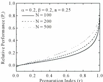
[image:5.595.337.508.84.221.2]

Using Equations (22) and (23) the first four figures (Figures 1 to 4) of this article have been drawn. These figures depict how one’s performance index ( ) de- pends on one’s preparation index (r).

Figure 3 clearly indicates that, negative marking in an examination, has very little effect on the probable per- formance of an examinee having an extremely good preparation.

We now recast Equation (14) as

 

   

1

f m QN f m

r

q q



 



 

 





QN

m f m

r P  C  _{ }

  (24)

where q and Q are already defined (Equations (20) and (21))









( ) 0.01 1 1

f m _ m n r  r __N n _ (25) Using the above two equations we have drawn Fig- ures 5 to 9. These curves depict the nature of variation of probability (Pm) as a function of m. The peak of any of

Figure 1. The variation of the relative performance (Pr) as a

function of preparation index (r) for different values of α. As r increases, Pr increases. For α = 0the variation is linear

(as evident from Equation (22)). For other values of α, the slope increases with r. At any fixed value of r, Pr decreases

as α increases.

Figure 2. The variation of the relative performance (Pr) as a

function of r for different values of β. As r increases, Pr in-

creases. At any value of r, Pr is larger for higher values of β.

[image:5.595.337.508.519.656.2]

These curves become closer to one another at higher values of r.

Figure 3. Relative performance (Pr) vs r plot for different

values of n. As r increases, Pr increases. At any particular

level of preparation r, Pr becomes smaller for higher values

of n. These curves become closer to one another at higher values of r. These curves converge in the direction of in- creasing r. At values of r close to 1 Pr becomes independent

[image:5.595.85.263.523.669.2]

of n.

Figure 4. This figure shows the variation of relative per- formance (Pr) as a function of preparation index (r) for dif-

ferent values of N. At any fixed value of r, Pr increases as N

Figure 5. This figure shows the variation of Pm as a function

[image:6.595.335.513.84.232.2]

of m for different values of α. As α decreases, the curve be- comes narrower, indicating smaller dispersion of the prob- able values of m. The peak of the curve, indicating the most probable value of m, becomes higher for smaller values of α. As α decreases the peak shifts towards higher values of m.

Figure 6. This figure shows the variation of Pm with m for

[image:6.595.83.263.304.443.2]

different β. As β increases, the curves become broader, in- dicating greater dispersion of the probable values of m. The peak of the curves, indicating the most probable value of m, becomes higher for smaller β. With increase in β, the peak shifts towards higher m.

Figure 7. Figure shows Pm-m variation for different n. As n

decreases, the curve becomes narrower, indicating smaller dispersion of the probable values of m. The peaks of these curves have the same height, although their positions are different. As n increase, the peaks shift towards smaller values of m, indicating smaller expectation value of m.

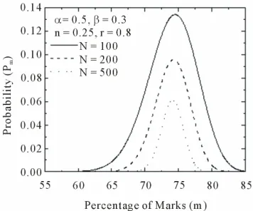
Figure 8. Variation of Pm as a function of m for different

values of N. The peaks of these curves appear at the same value of m, indicating the constancy of the most probable value of m. As N increases, the height of the curve decreases. For greater values of N, the probability (Pm) is smaller at all

[image:6.595.334.511.315.458.2]

values of m.

Figure 9. The variation of Pm with m for different values of r.

As r increases the peak shifts towards higher values of m. The most probable value of m increases as r increases. The curve becomes narrower and the peak height decreases with rise in r-value indicating ones true measure of prepa- ration for the examination.

these curves corresponds to the most probable value of

m.

In Figure 9 the narrowing of curves with rise in r in- dicates smaller dispersion of the probable values of m, implying smaller chances of deviation from the most probable value. A candidate, having a high score of r in the mock tests, is likely to acquire high marks in the final examination, with smaller deviation of probable values from the most probable m.

3. Limitations

[image:6.595.84.260.523.664.2]

termined from the mock test data and the estimation of performance has to be made for different values of β. The larger the value of , greater will be the validity and applicability of this approach where these parameters can be used to predict one’s performance. This model shows that one is likely to make better performance in examina- tions having larger number of questions. This depend- ence on N is a mathematical consequence that cannot generally be guessed from common sense. It has also been assumed that the process of attempting a question and its result is independent of attempting any other question. This assumption does not hold for linked com- prehension questions where, the process of attempting a question and its result depends on attempting other linked questions. In this regard a modification of our simple theory using the conditional probability [21] is required. Let the events of attempting successive ques- tions in a linked comprehension be A, B, C, etc. Then, according to the conditional probability [21] we have









  

P B A  P BA P A , (26)







  

P C B  P CB P B , (27) and so on.

These ideas can be incorporated for theoretical inter- ests. Calculations, based on such ideas, are likely to make this model so complicated that it would not be very useful to examinees preparing for competitive examina- tions. The mathematical simplicity in its present form is important in the sense that one can use this model suc- cessfully with considerable ease, for an estimation of performance, without making too much effort to grasp the underlying concept. The present analysis reveals im- portant and useful features, which one can’t discover just by intuition. It enables one to make an effective self- assessment, and thereby modify one’s plans, while pre- paring for an important examination.

REFERENCES

[1] D. K. Srinivasa and B. V. Adkoll, “Multiple Choice Questions: How to Construct and How to Evaluate?” In-

dian Journal of Pediatrics, Vol. 56, No. 1, 1989, pp. 69- 74.

[2] M. Tarrant and J. Ware, “Impact of Item-Writing Flaws in Multiple-Choice Questions on Student Achievement in High-Stakes Nursing Assessments,” Medical Education, Vol. 42, No. 2, 2008, pp. 198-206.

doi:10.1111/j.1365-2923.2007.02957.x

[3] P. Costa, P. Olivera and M. E. Ferrao, “Equalizacãâo de Escalas com o Modelo de Resposta as Item de Dois Parâmetros,” In: M. Hill, et al., Eds., Estatistica-da Teo-

ria à Pratica, Actas do XV Congresso Annual da So-

ciedade Portuguesa de Estatistica, Edicões SPE, 2008, pp. 155-166.

[4] P. Steif and J. Dantzler, “Astatics Concept Inventory:

Development and Psychometric Analysis,” Journal of

Engineering Education, Vol. 33, 2005, pp. 363-371. [5] P. Steif and M. A. Handsen, “Comparisons between Per-

formances in a Statics Concept Inventory and Course Examinations,” International Journal of Engineering

Education, Vol. 22, No. 3, 2006, pp. 1070-1076.

[6] E. Ventouas, D. Triantis, P. Tsiakas and C. Stergiopoulos, “Comparison of Examination Methods Based on Multiple Choice Questions,” Computers & Education, Vol. 54, No. 2, 2010, pp. 455-461.

doi:10.1016/j.compedu.2009.08.028

[7] D. Nicol, “E-Assessment by Design: Using Multiple- Choice Tests to Good Effect,” Journal of Further &

Higher Education,Vol. 31, No. 1, 2007, pp. 53-64. doi:10.1080/03098770601167922

[8] L. Thompson, “The Uses and Abuses of Multiple Choice Testing in a University Setting,”Annotated Bibliography Prepared for the University Centre for Teaching and Learning, University of Canterbury, Canterbury, 2005.

[9] P. Nightingale, et al., “Assessing Learning in Universi- ties,” Professional Development Centre, University of New South Wales, 1996, pp. 151-157.

[10] J. Heywood, “Assessment in Higher Education: Student Learning, Teaching Programmes and Institutions,” Jessica Kingsley Publishers, London, 2000.

[11] N. Falchikov, “Improving Assessment through Student Involvement: Practical Solutions for Aiding Learning in Higher and Further Education,” Routledge Falmer, Lon- don, 2005.

[12] D. Krathwohl, “A Revision of Bloom’s Taxonomy: An Overview,” Theory into Practice, Vol. 41, No. 4, 2002, pp. 212-218.doi:10.1207/s15430421tip4104_2

[13] S. Brown, “Institutional Strategies for Assessment,” In: S. Brown and A. Glasner, Eds., Assessment Matters in Higher

Education, SRHE and Open University Press, Bucking- ham, 1999, pp. 3-13.

[14] M. Culwick, “Designing and Managing MCQs,” Univer- sity of Leisester, The Castle Toolkit, 2002.

[15] S. Kvale, “Contradictions of Assessment for Learning in Institutions of Higher Education,” In: D. Boud and N. Falchikov, Eds., Rethinking Assessment in Higher Educa-

tion: Learning for the Longer Term, Routledge, London, 2007, pp. 57-71.

[16] M. Paxton, “A Linguistic Perspective on Multiple Choice Questioning,” Assessment and Evaluation in Higher Edu- cation,Vol. 25, No. 2, 2000, pp. 109-119.

doi:10.1080/713611429

[17] G. Gibbs and C. Simpson, “Conditions under Which As- sessment Supports Students’ Learning,” Learning and Teaching in Higher Education, Vol. 1, No. 1, 2004, pp. 3- 29.

[18] K. Scouller, “The Influence of Assessment Method on Students’ Learning Approaches: Multiple-Choice Ques- tion Examination versus Assignment Essay,” Higher Edu-

cation,Vol. 35, No. 4, 1998, pp. 453-472. doi:10.1023/A:1003196224280

Topics—Physics Education Research,Vol. 5, 2009, Arti- cle ID: 020103.

[20] N. G. Das, “Statistical Methods,” Tata McGraw-Hill Pub-lishing Company Ltd., New Delhi, 2008.

[21] A. M. Goon, M. K. Gupta and B. Das Gupta, “Funda- mentals of Statistics,” The World Press Pvt. Ltd., Kolkata,

1971.

[22] M. R. Spiegel, et al., “Schaum’s Outlines of Statistics,” 3rd Edition, McGraw Hill, New York, 1999.