Shedding Light on Non Binding Constraints in Linear Programming: An Industrial Application

(1)

http://www.scirp.org/journal/ajor ISSN Online: 2160-8849

ISSN Print: 2160-8830

DOI: 10.4236/ajor.2018.81005 Jan. 30, 2018 50 American Journal of Operations Research

Shedding Light on Non Binding Constraints in

Linear Programming: An Industrial Application

Alireza Tehrani Nejad Moghaddam

1*

, Thibault Monier

2

1_{Energy Economist, 22 Rue d’arcueil, Paris, France}

2_{Energy Economist, 10 Rue Mathis, Paris, France}

Abstract

In Linear Programming (LP) applications, unexpected non binding con-straints are among the “why” questions that can cause a great deal of debate. That is, those constraints that are expected to have been active based on price signals, market drivers or manager’s experiences. In such situations, users have to solve many auxiliary LP problems in order to grasp the underlying technical reasons. This practice, however, is cumbersome and time-consuming in large scale industrial models. This paper suggests a simple solution-assisted methodology, based on known concepts in LP, to detect a sub set of active constraints that have the most preventing impact on any non binding con-straint at the optimal solution. The approach is based on the marginal rate of substitutions that are available in the final simplex tableau. A numerical ex-ample followed by a real-type case study is provided for illustration.

Keywords

Linear Programming, Solution Interpretation, Non Binding Constraint, Decision Support

1. Introduction

Linear programming (LP) has found practical applications in all facets of busi-ness due to the computational efficiency of the simplex method and the

availa-bility of cheap and high-speed digital computers (for instance, see [1]). The oil

refining industry is an illustrative example of such applications since 1952 [2]. The rapid evolution of the easy-to-use software made model building and LP solving accessible to everyone. For instance, engineers are capable to construct refinery models by drawing graphically the process models, connecting them into sophisticated external simulators (for non linear computations), designing

How to cite this paper: Tehrani Nejad, A. and Monier, T. (2018) Shedding Light on Non Binding Constraints in Linear Pro-gramming: An Industrial Application. Amer-ican Journal of Operations Research, 8, 50-61.

https://doi.org/10.4236/ajor.2018.81005

Received: January 2, 2018 Accepted: January 27, 2018 Published: January 30, 2018

(2)

DOI: 10.4236/ajor.2018.81005 51 American Journal of Operations Research

intermediate tanks, blending final products and monitoring the storage capaci-ties. User interfaces are also configured to easily adapt the problem at hand into a multi-objective, multi-period or multi-location model. The commercial soft-ware imports the required input data from external sources, generates thousand of material and quality balance equations, points out data inconsistencies, de-bugs mathematical formulations, removes redundancies, linearizes the problem during the recursion passes (if necessary) and solves the problem in a fraction of time. Modern visualization technologies are also provided to report the solution in comprehensive manners.

Consequently, the seize and complexity of production planning models have increased to represent more accurately real operations. Today, we can optimize far more complex problems that we can understand. Powerful report generators provide numerical results without explaining “why the solution is what it is”. However, in strategic decision making and production planning, managers are

interested in whys not numbers [3]. Managers need to interrogate the model’s

output in terms of arbitrage and orientations before becoming confident in its utilization for decision making. The answer to these questions, which emerge from a deep understanding of the solution, is seldom evident from the output reports. Depending on users’ experience, ability and patience, analyzing the so-lution and preparing support for decision making can take up to several days. Surprisingly, this practical need continues to be neglected by the commercial op-timization software whose evolutions, driven primarily by computing speed and algorithms enhancement, have resulted in a new generation of LP users with a much less OR background.

The need to support the meaning of an optimal solution for non expert users is not new. During 1980 and 1990, Greenberg promoted and developed the project of Intelligent Mathematical Programming Systems (IMPS), initially mo-tivated by the US Department of Energy and sponsored by a consortium of

in-dustries [4][5][6][7][8]. The analysis module of IMPS, called ANALYZE,

in-cludes a collection of algorithms and rule-based heuristics to find causal sub-structures supporting analysis such as infeasibility diagnosis, suggestive reason-ing about redundancy and dual values interpretation associated with bindreason-ing constraints.

(3)

condition constraints such as the catalytic limitation which reacts inversely with the poly-aromatics content of the feed. Due to reliability issues related to up-stream logistics, the poly-aromatics content of the feed has been substantially increased. In this specific circumstance, the key production unit has reached its catalytic limitation before its hydraulic capacity constrain. This path-tracing analysis, that reveals the root cause of the non binding hydraulic constraint, re-quires advanced knowledge of the industrial process, the LP model scheme and its sensitivity to various input parameters. To the best of our knowledge, this kind of “why” questions related to non binding constraints have not been tackled in the literature.

The dual variables, which identify the bottlenecks of the model from the ob-jective function viewpoint, are not a proper tool for non binding constraint analysis. In Sections 4 and 5, we illustrate some cases where dual variables pro-vide counter intuitive indications. Moreover, the traditional sensitivity analysis on the right hand side parameters cannot neither explain why a given constraint is non binding. In the absence of any theoretical framework, users usually force the suspicious non binding constraints to operate at full capacity. Then, they in-vestigate by comparing the output results. Most often, much more auxiliary LP runs are required before grasping meaning and consistency of the solution beha-vior. This practice, however, is cumbersome and time-consuming when the problem is of anything else than trivial size and complexity and the expert re-sources are not available.

This practical-oriented paper is aimed to answer to the clear statement of the insights we wish to obtain from the model about why a given constraint is not active at the optimal solution. We suggest a solution-assisted procedure that can be considered as a kind of local sensitivity analysis carried out in a deterministic framework. The procedure tracks the marginal rate of technical substitutions (partial derivatives) between the slack variable of the given non binding con-straint and all the binding concon-straints in the final simplex tableau. Under the assumption of proportional perturbation, these marginal coefficients are trans-formed into elasticity measures capable to shed lights on directions which pre-vent a given non binding constraint from further saturation. These elasticities are comparable to the sensitivity measures of Samuelson’s comparative statics

which play an important role to support decision makers [9]. Under the non

(4)

industry. Finally, Section 7 concludes.

2. Definitions and Notations

Let us suppose the following profit maximization LP problem,

{

T

}

max c x Ax| ≤b x, ≥0 (1)

where, A is a given m n× linear technology matrix with full row rank. The

m-vector b represents the resource availabilities, called the right-hand-side (RHS)

terms, and the n-vector c represents the constant output market prices, called

the objective function coefficients. The n-vector x represents the non negative decision variables. The dual problem associated with model (1) can be formu-lated as follows,

{

T T

}

min b y A y d| − =c y, ≥0,d≥0 (2)

where, the m-vector y corresponds to the shadow input prices and the n-vector d

represents the opportunity (or reduced) cost associated with the primal variables. The dual constraint indicates that an equilibrium solution is achieved only when

the difference between marginal revenue c and marginal cost T

A y is

nonnega-tive for all the decision variables characterizing the production plan. If x is prim-al feasible,

(

y d,

)

is dual feasible and T

0

x d= , then they are primal-dual

op-timal solutions. Throughout this paper, we assume that the primal and dual problems are not degenerate so that the optimal variables are unique.

We partition the A technology matrix into a basic B and non basic component

N

A . The other vectors are also partitioned accordingly, c=

[

c cB, N

]

and

[

B, N

]

x= x x , where the basic variables x_B>0 and the non basic variables

0

N

x = . We denote I_B and I_N the sets of basic and non basic index

respec-tively. Rewriting the constraint equation of model (1), and pre-multiplying both sides by the inverse of the (non singular) basis matrix,

(

)

1 1

.

B N N

x =B b− − B A− x (3)

Relation (3) provides a simultaneous system of equations showing how all of

the basic variables xB are affected by marginal changes in the value of nonbasic

variables xN. In relation (3), the expression

(

)

1 N

B A− corresponds to the

ma-trix of marginal rate of technical substitution MRTS(xB,xN) between the non

ba-sic variables and all the baba-sic variables involved in the production plan [10].

(5)

instructions exist for Cplex and Xpress solvers. For other practical applications of the MRTS, please see Tehrani Nejad, 2007; Tehrani Nejad and Michelot, 2009;

Tehrani Nejad and Saint Antonin, 2014 [11][12][13].

3. Method

At the optimal solution, let us suppose that the i-th constraint is non binding.

Following relation (3), its positive slack variable xsi can be stated as below,

(

)

*

, ,

N

si si i si sk sk

k I

x x M x x x

∈

= −

∑

₍₄₎

where *

si

x is the optimal level of the basic slack variable and x_sk,k∈I_N refer to

non basic slack variables. In relation (4), the MRTS row-vector Mi

(

xsi,xsk

)

,

corresponds to the optimal adjustment of the basic slack variable

x

si in

re-sponse to marginal impulse in the RHS of the k-th binding constraint, bk. In

other words, Mi

(

xsi,xsk

)

is the rate at which xsi varies per unit increase in bk

at the optimal solution. These marginal rates reveal some sort of importance measure that can be used to rank the influence of the active constraints on the

saturation level of the ith non binding constraint. For notational convenience, let

(

,

)

ik i si sk

M =M x x . Since the marginal coefficients M_ik belong to the basis

in-verse 1

B− , they are free of sign. Depending on the optimal solution, negative or

positive Mik refer respectively to those active constraints whose relaxation

would increase or decrease the utilization rate of the i-th non binding constraint.

For the purpose of this paper, active constraints with negative Mik are of

inter-est.

That is evident that the Mik extracted from the final simplex tableau are not

directly comparable for two reasons. First, the LP constraints are usually ex-pressed in different units of measurement (ton, %, ˚C,...). Second, depending on

the constraint structure, some Mik might need adjustment. To circumvent this

limitation, we propose the following procedure that can be readily automated through post processors.

1) Extract the row-vector Mik associated with the i-th non binding

constraint from the final simplex tableau.

2) If the k-th active constraint is originally of type

∑

q xj j

∑

xi≤

α

, then the

associated Mik must be multiplied by

∑

xi (see [14]).

3) The sign of the Mik associated with an active greater-than-or-equal

con-straint must be reversed in order to be in line with a relaxation perturbation. 4) To render homogeneous the units of measurement and to scale the

varia-tions according to the size of the input constraints, each Mik must be converted

into a cross elasticity indicator Eik at the point of measure:

, ,

k

ik ik N

si

b

E M k I

x

= ⋅ ∈ ₍₅₎

(6)

elasticity Eik measures the responsiveness of the slack variable of the i-th non

binding constraint with respect to the marginal relaxation of the active con-straints individually. This local and individual sensitivity measurement, called critically importance measure in reliability analysis [9], can efficiently assist the user in a more in depth analysis of the LP solution.

5) Rank the Eik from the most negative values.

The most negative cross elasticity points out the active constraint that has the

most preventive impact on the saturation level of the i-th non binding constraint.

Then, the user has to evaluate the precision and the justification of the identified constraint. In practice, some of these active constraints can be relaxed after technical discussion with production engineers. Some others, however, remain truly the bottlenecks of the plant and have to be communicated to the managers for investment projects.

4. Non Linear Models

Industrial optimization models also include non linear constraints. These mod-els can be summarized as follows,

( )

{

T

}

max c x g x| ≤b h x, =0,x≥0 (6)

In relation (6), the constraints are segregated into linear g x

( )

and non

linear h x

( )

functions. The industrial practice consists in linearizing the non

linear functions using the first order Taylor expansion around a base point 0

x .

That is,

( )

( )(

)

{

T 0 0 0

}

max c x g x| ≤b h x, + ∇g x x−x =0,x≥0 (7)

This approximation is valid only in the neighborhood of the original point.

The base point _x0 and the derivatives

( )

0

g x

∇ _{must be reevaluated through}

recursion steps until the convergence criteria are reached. The LP problem (7) can be solved using the Simplex method where the relation (4) applies to its the non binding constraints.

5. Numerical Illustration

Let us suppose a stylized problem of producing gasoline xG, diesel xD and

fuel oil xF whose market prices are respectively $100, $150 and $55 per ton.

The producer can purchase five different grades of crude oil x x x x x1, 2, 3, 4, 5

whose market prices are respectively $90, $70, $80, $96, $75. We assume that the availability of crude oils x x2, 3 and x5 is limited to 75 tons and the

produc-tion capacity of diesel is limited to 150 tons. Due to corrosion issues, the sum of

crude x1 and x4 should remain lower than 30% of the total crude mix.

Processing each ton of crude generates respectively 0.3, 0.5, 0.3, 0.2 and 0.4 tons

of CO2. The regional authorities require that the total CO2 emissions should not

(7)

(

)

(

)

1 2 3 4 5

max 100 150 55 90 70 80 96 75

. .

0.40 0.40 0.45 0.16 0.35 0 Gasoline production 0.40 0.25 0.25 0.55 0.30 0 Diesel production 0.20 0.35 0.30 0.29 0.35

G D F

x x x x x x x x

s t

x x x x x x

+ + − − − − − + + + + − = + + + + − = + + + + − =

(

)

(

)

(

)

(

)

1 2 3 4 5 2

1 2 3 4 5

2 3 5

0 Fuel oil production 0.03 0.05 0.03 0.02 0.04 11.5 CO emissions 0.70 0.30 0.30 0.70 0.30 0 Corrosion limitation

75, 75, 75, D 150 Crude availability

x x x x x

x x x x

         + + + + ≤  ₋ ₋ ₊ ₋ _≤   ≤ ≤ ≤ ≤ 

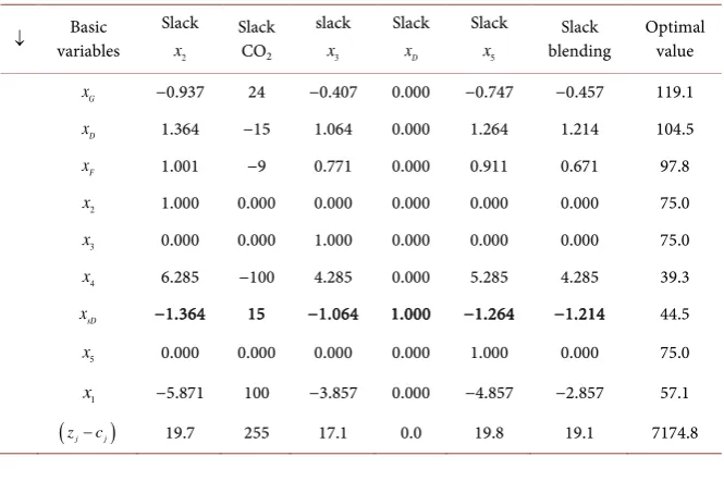
At the optimum, the total profit amounts to $7174.8. This level of perfor-mance is obtained by processing the five crude oils at 57.1, 75, 75, 39.3 and 75 tons respectively. The output products are consequently equal to 119.1, 104.5 and 97.8 tones for gasoline, diesel and fuel oil respectively. The crude oils 2, 3 and 5 are processed at their maximum availability leading to a positive

opportu-nity cost of $19.7, $17.1 and $19.8 respectively. Finally, the CO2 emissions and

corrosion blending constraints are both binding at optimum. The information

are summarized in Table 1 which contains a part of the final Simplex tableau.

The column to the immediate left indicates the basic activities as they appear

in the column of the basic index IB. Their optimal values are read in the most

right column. The first row corresponds to the slack variables associated with the binding constraints. The coefficients inside the tableau represent the MRTS be-tween the basic variables and non basic slack variables. The last row represents the dual optimal variables and the optimal value of the objective function.

Despite the higher relative price of diesel, its production capacity constraint is not fully utilized. This unexpected result, however, needs to be explained before recommending the production plan to refinery’s operators. The MRTS coeffi-cients that link the basic slack variable xsD to the binding constraints, i.e., the

[image:7.595.207.540.514.735.2]

bold row in Table 1, can provide valuable insights to this question. Following

Table 1. Part of the final simplex tableau.

↓ Basic variables Slack 2 x Slack CO2 slack 3 x Slack D x Slack 5 x Slack

blending Optimal value

G

x −0.937 24 −0.407 0.000 −0.747 −0.457 119.1

D

x 1.364 −15 1.064 0.000 1.264 1.214 104.5

F

x 1.001 −9 0.771 0.000 0.911 0.671 97.8

2

x 1.000 0.000 0.000 0.000 0.000 0.000 75.0

3

x 0.000 0.000 1.000 0.000 0.000 0.000 75.0

4

x _6.285 ₋₁₀₀ _4.285 _0.000 _5.285 _4.285 _39.3

sD

x −1.364 15 −1.064 1.000 −1.264 −1.214 44.5

5

x 0.000 0.000 0.000 0.000 1.000 0.000 75.0

1

x −5.871 100 −3.857 0.000 −4.857 −2.857 57.1

(8)

the suggested procedure in Section 3, we convert the extracted MRTS into an elasticity measure at the optimal solution. The blending constraint needs some

extra adjustment,

(

)

(

5

)

(

)

1

1.214 _i 0.3 45.5 2.57

E= −

∑

x = − . In words, at the

op-timal solution, 1% increase in the crude blending limitation would increase the

saturation level of the diesel production by 2.57%. Table 2 ranks the computed

elasticities from the most negative values.

Several interesting remarks are in order. First, the corrosion issue is the most preventive constraint for diesel production. Without this insight, the user should have relaxed all the binding constraints one by one in order to identify the most

responsive one. Second, contrary to its largest marginal value, the CO2

con-straint has a negative impact on diesel production: increasing the CO2 pollution

rights would alter the optimal crude processing by replacing crude 4 with crude

1 which has a higher CO2 content and a lower diesel yield. This optimal

substitu-tion, which is a consequence of the Rybczynski theorem in economics [10], leads

to increase the gasoline product (+24 tons) to the detriment of diesel (−15 tons). This counter intuitive example confirms the limitation of marginal values for non binding constraint analysis. Third, according to diesel production equation, crude oils 2 and 3 have the same average yield in terms of diesel output (%25). However, the computed elasticities reveal that crude oil 2 has a higher marginal yield and is, therefore, a more suitable candidate to increase the diesel output.

6. Case Study

In the previous section, we provided a very simple numerical example to detail the procedure. In this section, we apply the suggested methodology to a real-type refinery LP model which contains near to 5000 linear constraints and more than 7000 continuous variables. In this LP model, the constraints are categorized into material and quality balance constraints, product specification constraints, crude availability constraints and process units capacity constraints. The linear objec-tive function consists in maximizing the net profit of the oil refining operations

(for more details, see Tehrani Nejad and Saint Antonin [15]). Cplex is the used

solver.

6.1. Model Overview

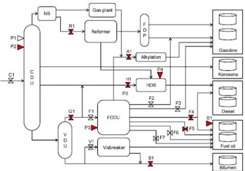
The general scheme of the model is given in Figure 1. In non technical words,

the crude distillation unit (CDU) separates crude oils into various fractions ac-cording to their boiling points. Light fractions are used to make gasoline and naphtha whilst middle fractions are used to produce kerosene and diesel. The heaviest fractions are sent to vacuum distillation unit (VDU) to produce vacuum distillate and vacuum residue. The major part of vacuum residue is fed to a

Table 2. Sensitivity importance measures.

Blending Crude 2 Crude 5 Crude 3 CO2 emissions

(9)

[image:9.595.60.539.66.400.2]

Figure 1. Oil refinery scheme.

visbreaker, to reduce the viscosity of the fuel oil products. The vacuum distillate is converted by a fluid catalytic cracker unit (FCCU) to a gasoline blending component and light cycle oil for blending into the diesel pool. Here, the FCCU is combined with an Alkylation unit to produce high value gasoline components called alkylate. The sulfur specifications for gasoline, middle and heavy oil products require the use of a hydro-desulfurization unit (HDS). On the other side, a reforming unit converts low-octane naphthas into high-octane gasoline blending components. Most often, reformer’s output is separated into light and heavy components by a fractionation unit called FDP. The oil product categories considered are propane, butane, naphtha, gasoline, jet fuel, diesel, heating oils, heavy fuel oils and different bitumen grades.

6.2. Results and Discussion

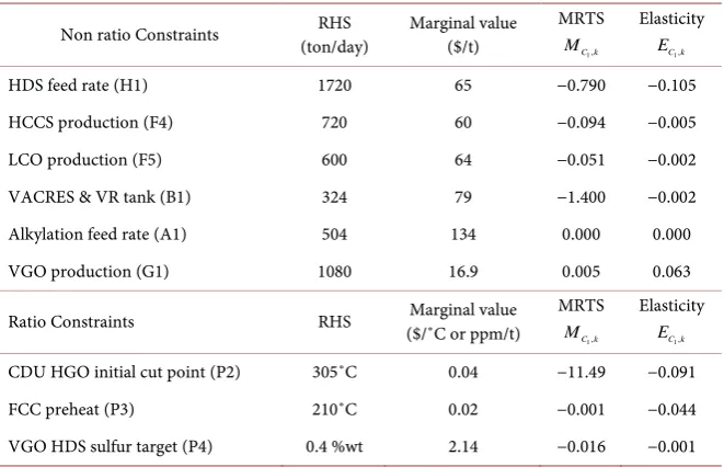
Based on market indicators, the manager expects the crude distillation unit (CDU) to be fully utilized. However, the optimal solution recommends an

aver-age utilization rate of 91.5%. Table 3 summaries the main active constraints at

the optimal solution. These active constraints are illustrated by bold arrows in

(10)

[image:10.595.209.540.88.301.2]

Table 3. Marginal values, MRTS and elasticities measures.

Non ratio Constraints _(ton/day)RHS Marginal value _($/t) MRTS

1,

C k

M

Elasticity

1,

C k

E

HDS feed rate (H1) 1720 65 −0.790 −0.105

HCCS production (F4) 720 60 −0.094 −0.005

LCO production (F5) 600 64 −0.051 −0.002

VACRES & VR tank (B1) 324 79 −1.400 −0.002

Alkylation feed rate (A1) 504 134 0.000 0.000

VGO production (G1) 1080 16.9 0.005 0.063

Ratio Constraints RHS _{($/˚C or ppm/t)}Marginal value MRTS

1,

C k

M

Elasticity

1,

C k

E

CDU HGO initial cut point (P2) 305˚C 0.04 −11.49 −0.091

FCC preheat (P3) 210˚C 0.02 −0.001 −0.044

VGO HDS sulfur target (P4) 0.4 %wt 2.14 −0.016 −0.001

elastisities Eik between the mentioned active constraints and the slack variable

of the CDU capacity constraint. The results are reported in the two last columns of Table 3.

Several remarks are in order. First, the HDS feed rate constraint is directly identified to be the most preventing constraint with respect to the CDU throughput. We verified this result by increasing individually the RHS of the

ac-tive constraints reported in Table 3. By relaxing only the HDS capacity up to

60%, the utilization rate of the crude unit increases steeply from 91.5% to 96.6%, and then flattens. Second, given the high marginal values of the gasoline-related

units, i.e., Alkylation and the FCC effluents (HCCS and LCO), the LP practioner

would have been most plausibly disoriented by first inspecting those constraints. Third, although the Alkylation unit has the highest marginal value, its cross elas-ticity with respect to crude distillation unit is zero. That simply implies having more Alkylation would significantly increase the overall net margin of the refi-nery without impacting the crude intake amount. Forth, the relative high mar-ginal value of the HDS capacity constraint confirms that the low utilization rate of the crude unit, suggested by the optimal solution, is not simply due to low price effects.

7. Conclusion

(11)

The distinguished feature of this approach is that it requires no more informa-tion than what is provided by the final simplex tableau. A numerical example as well as a real-type oil refining case study was provided to illustrate the procedure. The simplicity of this method, we believe, constitutes its elegance.

Acknowledgments

Without involving them in any possible error, the first author would like to ex-press his gratitude to Quirino Paris, Harvey Greenberg and Nastaran Manou-chehri for their valuable comments on this paper.

References

[1] Bixby, R. (2012) Documenta Mathematica. Extra Volume ISMP, 107-121.

[2] Charnes, A., Cooper, W.W. and Mellon, B. (1952) Blending Aviation Gasoline—A Study in Programming Interdependent Activities in an Integrated Oil Company.

Econometrica, 20, 135-139. https://doi.org/10.2307/1907844

[3] Geoffrion, A. (1976) The Purpose of Mathematical Modeling Is Insight, Not Num-bers. Interfaces, 7, 81-92. https://doi.org/10.1287/inte.7.1.81

[4] Greenberg, H.J. (1987) ANALYZE: A Computer-Assisted Analysis System for Li-near Programming Model. Operational Research Letters, 76, 249-255.

https://doi.org/10.1016/0167-6377(87)90057-5

[5] Greenberg, H.J. (1991) Intelligent Analysis Support for Linear Programs. Comput-ers Chemical Engineering, 16, 659-673.

https://doi.org/10.1016/0098-1354(92)80015-2

[6] Greenberg, H.J. (1991) A Primer for ANALYZE: A Computer-Assisted Analysis System for Mathematical Programming Models and Solutions. Operations Research Society of America, Baltimore, MD.

[7] Greenberg, H.J. (1993) How to Analyze the Results of Linear Programs, Part 2: Price Interpretation Interfaces. 23, 97-114. https://doi.org/10.1287/inte.23.5.97

[8] Greenberg, H.J. (1996) A Bibliography for the Development of an Intelligent Ma-thematical Programming System. Annals of Operations Research, 65, 55-90.

https://doi.org/10.1007/BF02187327

[9] Borgonovoa, E. and Plischke, E. (2016) Sensitivity Analysis: A Review of Recent Advances. European Journal of Operational Research, 248, 869-887.

https://doi.org/10.1016/j.ejor.2015.06.032

[10] Paris, Q. (2013) An Economic Interpretation of Linear Programming. Revised Edi-tion, Palgrave Mcmillan.

[11] Tehrani Nejad, M.A. (2007) Allocation of CO2 Emissions in Petroleum Refineries to Petroleum Joint Products: A Linear Programming Model for Practical Application.

Energy Economics, 29, 974-977. https://doi.org/10.1016/j.eneco.2006.11.005

[12] Tehrani Nejad, M.A. and Michelot, Ch. (2009) A Contribution to the Linear Pro-gramming Approach in Joint Cost Allocation: Methodology and Application. Eu-ropean Journal of Operational Research, 197, 999-1011.

(12)

DOI: 10.4236/ajor.2018.81005 61 American Journal of Operations Research [14] Rosenthal, R.E. (2015) GAMS, a User’s Guide. GAMS Development Corporation,

Washington DC.

http://www.scirp.org/journal/ajor

: 10.4236/ajor.2018.81005

http://creativecommons.org/licenses/by/4.0/

. https://doi.org/10.2307/1907844

https://doi.org/10.1287/inte.7.1.81

https://doi.org/10.1016/0167-6377(87)90057-5

https://doi.org/10.1016/0098-1354(92)80015-2

. https://doi.org/10.1287/inte.23.5.97

https://doi.org/10.1007/BF02187327

7. https://doi.org/10.1016/j.eneco.2006.11.005

28. https://doi.org/10.1007/s11367-013-0634-9