University of Warwick institutional repository: http://go.warwick.ac.uk/wrap
This paper is made available online in accordance with
publisher policies. Please scroll down to view the document
itself. Please refer to the repository record for this item and our
policy information available from the repository home page for
further information.
To see the final version of this paper please visit the publisher’s website.
Access to the published version may require a subscription.
Author(s): E. GUYEZ, J.-B. FLOR and E. J. HOPFINGER
Article Title: Turbulent mixing at a stable density interface: the variation
of the buoyancy flux–gradient relation
Year of publication: 2007
Link to published version: http://dx.doi.org/
10.1017/S0022112007004958
J. Fluid Mech.(2007),vol.577,pp.127–136. c 2007 Cambridge University Press doi:10.1017/S0022112007004958 Printed in the United Kingdom
127
Turbulent mixing at a stable density interface: the
variation of the buoyancy flux–gradient relation
E. G U Y E Z†, J. - B. F L O RA N D E. J. H O P F I N G E R
LEGI-CNRS-UJF, BP 53, 38041 Grenoble Cedex 9, France
(Received27 July 2006 and in revised form 19 January 2007)
Experiments conducted on mixing across a stable density interface in a turbulent Taylor–Couette flow show, for the first time, experimental evidence of an increase in mixing efficiency at large Richardson numbers. With increasing buoyancy gradient the buoyancy flux first passes a maximum, then decreases and at large values of the buoyancy gradient the flux increases again. Thus, the curve of buoyancy flux versus buoyancy gradient tends to be N-shaped (rather than simply bell shaped), a behaviour suggested by the model of Balmforth et al. (J. Fluid Mech. vol. 428, 1998, p. 349). The increase in mixing efficiency at large Richardson numbers is attributed to a scale separation of the eddies active in mixing at the interface; when the buoyancy gradient is large mean kinetic energy is injected at scales much smaller than the eddy size fixed by the gap width, thus decreasing the eddy turnover time. Observations show that there is no noticeable change in interface thickness when the mixing efficiency increases; it is the mixing mechanism that changes. The curves of buoyancy flux versus buoyancy gradient also show a large variability for identical experimental conditions. These variations occur at time scales one to two orders of magnitude larger than the eddy turnover time scale.
1. Introduction
In geophysical flows, stable density stratification can drastically reduce the vertical transfer of heat and mass. In the upper layer of the ocean for instance the turbulence produced by the wind stress forms a mixed layer bounded below by a density interface known as the thermocline. The depth of this mixed layer depends on the intensity of the wind stress and the density gradient. Density interfaces, separated by mixed layers, also exist at greater depths, which are a result of internal turbulence production and consequent mixing events. Experiments on mixed layer deepening by turbulence produced at the boundary of a stratified layer have been able to establish the deepening rate as a function of stratification or, more generally, the buoyancy flux–buoyancy gradient relation (see for example: Turner 1973; Kato & Phillips 1969; Linden 1979; E & Hopfinger 1986; Hannoun & List 1988; Fernando 1991). The buoyancy flux–gradient relation usually exhibits the characteristic bell-shaped curve suggested by Phillips (1971) and Posmentier (1977). Internal turbulence generated by shear-unstable stratified flows and related mixing processes have been reviewed by Peltier & Caulfield (2003), who pay particular attention to the streamwise vortices associated with convective instability, and suggest that these secondary vortices have an important effect on the mixing efficiency in the late-stage flow evolution, i.e. for large Richardson numbers.
An interesting example of internal mixing is the laboratory experiments by Park, Whitehead & Gnanadeskian (1994) in which a vertical rod is moved through a stably stratified fluid layer. These experiments demonstrate, for a given kinetic energy input and sufficiently large buoyancy gradient, the rapid formation of mixed layers separated by sharp density interfaces. The experiments with linearly stratified Taylor– Couette flow (Caton, Janiaud & Hopfinger 2000) also showed rapid formation of layers separated by interfaces. This behaviour is in agreement with the theoretical model of Phillips (1971) and Posmentier (1977) which suggests a decreasing buoyancy flux with increasing buoyancy gradient. Since a perturbation of the density profile is amplified this is referred to as unstable behaviour of the flux–gradient relation; the resulting layer formation is the cause of a continuous weakening of the buoyancy flux. The flux–gradient curve has an asymmetric bell-shaped form with maximum flux at intermediate values, and a decreasing flux with increasing buoyancy gradient. In the Phillips–Posmentier model the interface steepening is unlimited since it does not take into account a diffusive mechanism. It has been pointed out by Barenblattet al.
(1993) and Balmforth, Llewellyn Smith & Young (1998), that the Phillips–Posmentier model is also mathematically ill-posed because the linearized diffusion equation has a negative diffusivity.
Balmforthet al.(1998, referred to herein as BLY), proposed a model that includes turbulent eddy diffusion of kinetic energy and of buoyancy, and is based on a buoyancy-dependent mixing length. Thus the decreasing flux–gradient relation at large buoyancy gradient is limited and the mathematical ill-posedness eliminated. At large Richardson numbers, i.e. when the buoyancy gradientBz is large, the mixing length is a function of the buoyancy gradient Bz in the form l∝(e/Bz)1/2, such that ld
wheredis the turbulent eddy scale fixed by the device geometry. This mixing length is proportional to the Ozmidov length. The choice of energy production is crucial in the BLY model. Of most interest is the ‘equipartition’ model for which, in the absence of stratification, the eddy speede1/2adjusts, on the eddy turnover time scalel/e1/2, to the
characteristic velocityU of the stirring device. The energy production available for the mixing isαe1/2U2/ l, whereαis an adjustable parameter in the model. According to this
model the asymmetric bell-shaped curve changes to an N-shaped curve, with the flux increasing again at large buoyancy gradients, i.e large Richardson number. In BLY this increasing flux corresponds to a strongly stable buoyancy gradient at mixing fronts that gradually reduce the buoyancy gradient to a thin interface. However, this high-Richardson-number increase in buoyancy flux has never been observed in experiments. The BLY model was partly motivated by the experiments of Park et al. (1994). These experiments indicate that the flux Richardson number, Rif, also known as mixing efficiency and defined by the ratio of the change in potential energy to kinetic energy input, reaches a low-Rif plateau at large values of the Richardson number,
Ri=gρδ/ρU¯ 2, whereδis the interface thickness,ρthe density across the interface
and ¯ρthe mean density,g gravity andU the speed of the vertical rod moved through the fluid. Furthermore, the experiments show a large variability of flux Richardson number with energy input.
It is of interest to investigate the flux–buoyancy-gradient relation in the light of the BLY model by considering only one interface under well-controlled conditions that allow the completeRif–Ri curve to be obtainted. These conditions were achieved in
Turbulent mixing at a density interface 129
is reduced and will be a small fraction of the gap width d. The strength of the overturning eddies is proportional toΩ, the rotation speed of the inner cylinder. This suggests that the conditions of ‘equipartition’ in the sense of the BLY model might be satisfied in the Taylor–Couette flow device.
In §2 we present details of the experimental set-up and measurement techniques. Section 3 contains the results, giving the entrainment rate and mixing efficiency as a function of the Richardson number for a fixed Reynolds number and initial, interfacial buoyancy jumps varying by two orders of magnitude. The sharpening of the interface and the relaxation to a finite thickness are highlighted by the experiments. The different mechanisms of mixing are illustrated using laser-induced fluorescence (LIF) visualizations. Conclusions and discussions are presented in§4.
2. Experimental conditions
The experiments were conducted in the large-gap Taylor–Couette apparatus used by Boubnov & Hopfinger (1997) for the study of the effect of a linear density stratification on the instability and flow structure. The inner and outer radii were respectively rint= 15 cm and rext= 20 cm and the gap width was d= 5 cm. The total height was 70 cm and the gap was filled with fresh and salty water toh ≈62 cm with the density interface positioned at mid-height. This allowed three pairs of turbulent vortices to exist above and below the interface. As boundary conditions a free surface was used, and to reduce end effects on the turbulent vortex structure, the inner half of the bottom boundary rotated with the inner cylinder.
The initial density interface thickness was about 2 cm and the initial buoyancy difference was 0.006< Bi<1.32 cm s−2(B=gρ/ρ¯). The Reynolds numberRe =
Ωrintd/ν was kept constant atRe= 3409.
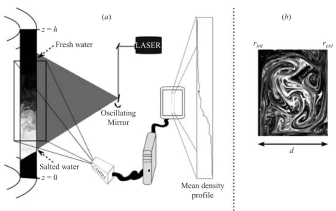
The density was measured with the LIF technique. The fluorescent dye (Rhodamine 6G) was excited by a 5 W argon laser at 515 nm and emitted at a wavelength>530 nm. A known concentration of fluorescent dye was dissolved in the denser layer and the evolution of its concentration in the gap cross-section followed in time. The dye concentration was usually about 10−6mol l−1 and the resolution was better than 1 %
of the initial concentration. The arrangement is shown schematically in figure 1(a) and figure 1(b) shows a cross-section of the turbulent eddy structure at Re= 3409 in a homogeneous fluid.
Turbulent eddy velocities were measured, using the particle image velocimetry (PIV) method and an algorithm developed by Fincham & Spedding (1997) and Fincham & Delerce (2000); for each turn of the inner cylinder 10 PIV measurements were made. Slightly heavy particles (Argosol) of 70µm diameter and density 1.04 g cm−3 were
seeded in the fluid and remained equally distributed over the entire fluid depth for approximately 2 hours. A laser illuminated the particles over a 1 cm thick vertical slice from the side, and images were taken with a 1000×1000 pixel B&W camera. The r.m.s. eddy velocity thus obtained is Uϑ= 0.76 cm s−1 atRe= 3409.
3. Results
3.1. Entrainment rate
z = h
z = 0 Salted water
Fresh water
(a) (b)
Oscillating Mirror
Mean density profile
rint rext
d
LASER
[image:5.493.85.421.53.264.2]CAMERA
Figure 1.(a) Sketch of the experimental set-up with the gap containing dyed salty water,
the position of the laser sheet, and a measured density profile of a diffused interface. (b) Cross-section of the turbulent flow structure atRe= 3409 in a homogeneous fluid.
or both sides of the interface. The buoyancy flux was calculated from the temporal evolution of the dye concentration, which is proportional to the density as indicated in figure 1. The density profile was averaged over the gap width and over one rotation period, and the density flux was then determined from the integral
F(z, t) =
h
z
∂ρ(z, t)
∂t dz. (3.1)
At the boundaries z= 0 and z=h the flux is zero so that when the interface is thin and bounded by mixed layers, the flux decreases linearly above and below the interface. Since the interface is free to move and the density may not be completely uniform in the mixed layers, there is in general a deviation from a linear variation. Furthermore, when the buoyancy gradient becomes small, the interface is no longer sharp (as indicated in figure 1) and no mixed layers exist. The flux can be expressed in terms of an entrainment velocityUe across the interface in the form
F(zm, t) =ρ(t)Ue(t), (3.2)
where the density difference,ρ, varies in each experiment from the initial valueρi
to zero at the end of the experiment, and the integration is from the interfacezm to the surface h. The rate of decrease of the density difference was initially very small so that for the case under consideration withRe= 3409 a typical experiments lasted 24 hours or more. Therefore, the density evolution can be considered quasi-steady. The buoyancy flux and buoyancy gradient are made dimensionless by the kinetic energy input. The instantaneous overall Richardson number, based on the eddy size
dϑ and the r.m.s. turbulent velocity, is defined by
Ri0(t) =
dϑ(t)B(t)
Turbulent mixing at a density interface 131
10–1
10–2
10–3
10–4
100 101 102 103
E
Ri0
Ri0–3/2
[image:6.493.109.375.60.281.2]Ri0–1
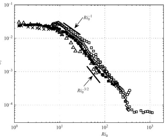
Figure 2. Entrainment coefficient E versus Richardson number Ri0 at Re= 3409: 䊐,
Bi= 1.32; 䊊, 䉫, Bi = 0.35; 䊏, Bi= 0.21; , Bi= 0.067; ×, Bi= 0.017 (in m s−2). Each point corresponds to a mean value of approximately 50 data points.
and the entrainment coefficient by
E(t) = Ue(t)
Uϑ , (3.4)
where Uϑ = 0.76 cm s−1 and dϑ(t) = (h−zm(t))/6≈5 cm. These quantities,
cha-racteristic of a turbulent eddy, allow comparison with other experiments.
The behaviour of E versusRi0for Re= 3409 and different values ofBi is shown
in figure 2. The slopes Ri−01 and Ri−03/2, often observed (see the review by Fernando 1991), are indicated for comparison. From one experiment to another and for different sub-ranges ofRi0there is a significant variability in slope. In the range 20<Ri0<200
the least-square mean slope is Ri−1.32
0 . The interesting point is that whenRi0 is large
the entrainment coefficient reaches a plateau and even increases with increasing Richardson numbers. This behaviour is not due to the adjustment of the initial interface thickness that takes place on a time scale one or two orders of magnitude less than the variation in entrainment rate (see figure 4), but rather to a change in mixing length scale as proposed by BLY. In the other limit of small Ri0, the entrainment
coefficient reaches a constant value of aboutE≈2×10⁻². This value is less than that
obtained for oscillating grid turbulence, where E≈0.2 (E & Hopfinger 1986), but compares well with the shear-induced turbulent flows reviewed by Fernando (1991).
3.2. Mixing efficiency
0 5 10 15 20 25 30 35
100 101 102 103
Ri0 Rif
[image:7.493.127.387.54.279.2](%)
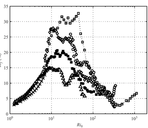
Figure 3.Mixing efficiency expressed by the flux Richardson number Rif as a function of
the overall Richardson number Ri0. The symbols correspond to the same initial buoyancy
jumps as in figure 2.
with other experiments. The flux Richardson numberRif is then
Rif(t) =
dϑ(t)B(t)Ue(t)
Uϑ3 =Ri0
Ue
Uϑ. (3.5)
In figure 3 the flux Richardson number is plotted as a function ofRi0 for the same
initial buoyancy jumps as in figure 2. In this presentation the increase in buoyancy flux at largeRi0 is more pronounced. There is also a large variability in mixing efficiency;
in particular the maximum value varies between about 15 % and 30 %, a variation similar to what is observed in other experiments (see Linden 1979). A 30 % mixing efficiency is generally accepted as a maximum value; most of the turbulent kinetic energy is dissipated by viscosity (Sherman, Imberger & Corcos 1978). Furthermore, the increase in mixing efficiency at large values of Ri0 does not occur at the same
value of Ri0 (or B). Experiments performed for the same initial density step
(Bi = 0.35 m s−2, symbols
◦
and in figures 2 and 3) show local overlaps, but forlargeRi0 a clear increase is observed in one experiment (
◦
) whereas in the other ()a plateau occurs at large B, suggesting that for larger values of B the mixing efficiency would increase, as is the case in experiment () withBi = 1.32 m s−2.
The value of the mixing efficiency depends on the definition of the rate of kinetic energy supply. Park et al. (1994) use, for instance, the work of the displaced rod per unit time which is difficult to convert to local turbulent kinetic energy supply as used in the present experiments. Local turbulent kinetic energy supply per unit time is more universal and allows comparison of different experimental conditions. Also,U3
ϑ
is proportional to the energy dissipation rate.
3.3. Evolution of the density interface
In figures 4(a) and 4(b) we show for Bi= 0.35 and 1.32 m s−2 the variations of the
Turbulent mixing at a density interface 133
36
(a) (b)
30
24
18
12
6
0 0.1 0.2 0.3 0.4 0.5 0.6 0.7 0.8
(× 104)
0.15 0 0.30 0.45 0.60 0.75 0.90 0.15 0 0.30 0.45 0.60 0.75 0.90
t/Tϑ
360 330 301 274 250 220 183 130 67 976 791 607 480 394 297 134
Rif
(%)
Ri0 Ri0
36 30 24 18 12 6
0 0.5 1.0 1.5 2.0 2.5 3.0 3.5
(× 104)
t/Tϑ
[image:8.493.53.428.61.281.2]Ri f (%) δ / d δ / d
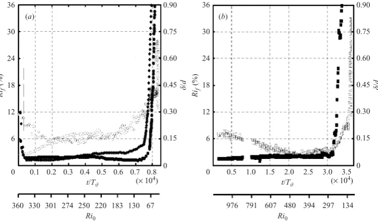
Figure 4. Evolution of the non-dimensional interface thickness (filled symbols; right scale)
and of the flux Richardson number Rif (open symbols; left scale), for (a) Bi = 0.35 m s−2 for both experiments, and (b)Bi= 1.32 m s−2. The decrease of the initial interface thickness (i.e. fromt/Tϑ = 0 to about 300) corresponds to the initial adjustment. The symbols are the same as in figure 2.
The initial interface thickness depends on the filling procedure and on molecular diffusion; its value is δ/d <0.4. When the experiment was started at time t= 0, the interface thickness decreased rapidly in a timet/Tϑ≈300 to a value ofδ/d≈0.05; this thickness corresponds to 5 pixels (1 pixel = 0.5 mm). The mixing efficiency decreases slightly in this initial adjustment (figure 4a), and then continues to decrease during about 103to 104eddy turnover times (depending on∇Bi) while the interface thickness
remains practically constant. Then, the mixing efficiency increases and when it approaches its maximum the interface thickness increases rapidly.
This evolution is typical of the behaviour at large Bi and gives an indication of the sharpness of the interface and the slow mixing process (long time scales). It is worthwhile to stress again, as is clearly demonstrated in figure 4, that the minimum mixing efficiency is not reached at the same value of Ri0. The experiment
with Bi= 0.35 m s−2 (figure 4a) has a minimum mixing efficiency in one case (
◦
) atRi0≈300 and in the other () at around 350. The latter follows more closely the
exper-iments withBi= 1.32 m s−2 (figure 4b, ) which show a clear increase atRi
0>480.
The question arises of whether the increase in mixing efficiency at large Ri0 is due
to molecular diffusion or to a mechanism proposed by BLY, i.e. a decrease in effective eddy turnover time scale that is l/e1/2 rather thand/Uϑ. It is well known that when
Ri0 is very large, the buoyancy flux–gradient curve flattens out (Turner 1973) and no
longer depends onRi0 but rather on the P´eclet number, here defined asP e=le1/2/D,
where D is the molecular diffusivity of salt equal to 1.37×10⁻⁵. Taking e1/2≈Uϑ
and l = δ 0.05d (figure 4), gives P e = 1.4×10⁴. The contribution of molecular
diffusion to the average buoyancy flux at large Ri0 is not entirely negligible but
(a) (b) (c)
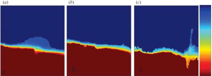
Figure 5.Time sequence of video frames of the interface for (a) Ri0 = 335, Rif= 8 %,
(b) Ri0= 312, Rif= 5 %, (c) Ri0= 128, Rif= 8 %. The initial buoyancy jump is Bi= 0.35 m s−2. The colour bar at the right represents the density scale with red higher, and blue
lower density water. The contrast is increased to optimize the visualization of the interface.
asFE=KρUϑRi0−3/2, the expression for the total dimensionless flux is then
E =KRi0−3/2
1 + D
KUϑδRi
3/2 0
. (3.6)
The coefficient K≈1, evaluated from figure 2 at Ri0≈100 when the diffusive flux
is negligible. With δ= 0.05d (figure 4), we get D/(KUϑδ)≈1/P e≈7×10⁻⁵. This
requiresRi0>103 for the entrainment curve to flatten out due to molecular diffusion;
it would never increase with increasingRi0. The flattening in buoyancy flux observed
in the experiments is, therefore, not due to molecular diffusion.
Figure 5 shows interface mixing events for∇Bi = 0.35 m s−1and forRi
0= 335 where
the mixing efficiency Rif= 8%, for Ri0= 312 where Rif= 5%, and for Ri0= 128
where Rif has increased again to 8%. For the largest Ri0 (figure 5a) there are
occasional overturning events. At minimum mixing efficiency (figure 5b) the interface is fuzzy and then atRi0= 128 mixing occurs mainly near the outer cylinder, causing
large vertical excursions. It is plausible that the overturning event at large Ri0 is
caused by energetic, smaller eddies in the sense of the BLY model.
4. Conclusions
The present experiments on mixing across a density interface in stratified Taylor– Couette flow show clearly a lower limit of mixing efficiency with an increase at large buoyancy gradient. This is the first time that, at largeRi0, an increase has been
Turbulent mixing at a density interface 135
buoyancy gradients is associated with a change in mixing mechanism (figure 5) from random scraping to small-scale overturning events.
Another novel feature of the present experiments is the large variability in mixing efficiency for identical flow conditions. This demonstrates the randomness of mixing in stratified fluids. In an identical experiment with the same initial density difference, there is a significant variation in local slopes (see figure 2, symbols
◦
and ). A possible explanation is that mixing events are intermittent such that the adjacent turbulent eddies are intermittently affected by stratification and readjust on a slow time scale.The Taylor–Couette configuration has an analogy with mixing by Langmuir circulation. The planes of symmetry of the Langmuir cells are here replaced by the cylinder walls. In Langmuir circulation mixing models, mixing is arrested when the Froude number is O(1) (Li, Garrett & Zahariev 1995; Li & Garrett 1997). This Froude number corresponds, according to the present results, to the maximum mixing efficiency. Another example of coherent vortices is Ekman rolls which develop in the planetary boundary layer as persistent counter-rotating vortices that are aligned with the mean wind.
The authors acknowledge the technical assistance of Pierrre Carecchio and Joseph Virone. E. Guyez acknowledges a DGA fellowship. This study has been supported by SHOM (the french Navy hydrographic and oceanographic institute) through the program MOUTON (operational oceanography for coastal areas) under contract 02.87.028.00.470.29.25.
R E F E R E N C E S
Balmforth, N. J., Llewellyn Smith, S. G. & Young, W. R. 1998 Dynamics of interfaces and
layers in a stratified turbulent fluid.J. Fluid Mech.428, 349–386 (referred to herein as BLY).
Barenblatt, G. I., Bertsch, M., Del Passo, R., Prostokishin, V. M. & Ughi, M. 1993 A
mathematical model of turbulent heat and mass transfert in stably stratified shear flow. J. Fluid Mech.253, 341–358.
Boubnov, B. M. & Hopfinger, E. J.1997 Experimental study of circular Couette flow in a stratified
fluid.Fluid Dyn.32(4), 520–528.
Caton, F., Janiaud, B. & Hopfinger, E. J. 2000 Stability and bifurcations in stratified Taylor–
Couette flow.J. Fluid Mech.419, 93–124.
E, X. & Hopfinger, E. J. 1986 On mixing across an interface in stably stratified fluid. J. Fluid
Mech.166, 227–244.
Fernando, H. J. S.1991 Turbulent mixing in stratified fluids.Annu. Rev. Fluid Mech.23, 455–493. Fincham, A. & Delerce, G. 2000 Advanced optimization of correlation imaging velocimetry
algorithms.Exps. Fluids29(7), 13–22.
Fincham, A. & Spedding, G. R.1997 Low cost, high resolution dpiv for measurement of turbulent
fluid flow.Exps. Fluids23(6), 449–462.
Hannoun, I. A. & List, E. J. 1988 Turbulent mixing at an shear-free density interface. J. Fluid
Mech.189, 211–234.
Kato, H. & Phillips, O. M. 1969 On the penetration of a turbulent layer into stratified fluid.
J. Fluid Mech.37, 643.
Li, M. & Garrett, C.1997 Mixed layer deepening due to Langmuir circulation.J. Phys. Oceanogr. 27, 121–132.
Li, M., Garrett, C. & Zahariev, K. 1995 Role of Langmuir circulation in the deepening of the
ocean surface mixed layer.Science270, 1955–1957.
Linden, P. F.1979 Mixing in stratified fluids.Geophys. Astrophys. Fluid Dyn.13, 3–23.
Park, Y. G., Whitehead, J. A. & Gnanadeskian, A. 1994 Turbulent mixing in stratified fluids:
Peltier, W. R. & Caulfield, C. P.2003 Mixing efficiency in stratified shear flows.Annu. Rev. Fluid
Mech.35, 135–167.
Phillips, O. M.1971 Turbulence in a strongly stratified fluid- is it unstable? Deep Sea Res. 19,
79–81.
Posmentier, E. S. 1977 The generation of salinity finestructure by vertical diffusion. J. Phys.
Oceanogr.7, 298–300.
Sherman, F. S., Imberger, J. & Corcos, G. M. 1978 Turbulence and mixing in stably stratified
waters.Annu. Rev. Fluid Mech.10, 267.
Turner, J. S.1968 The influence of molecular diffusivity on turbulent entrainment across a density
interface.J. Fluid Mech.33, 639.