Generating physics based 1D surrogate models from 2D model results

Full text

(1)Master Thesis Generating physics-based 1D surrogate models from 2D model results. Ilia Awakimjan.

(2) Cover image: Visualisation of FM2PROF output for a section of the 2D Flexible Mesh Waal model. White lines represent flow-links that have been categorised as belonging to the floodplain and black ones as belonging to the main channel..

(3) Master Thesis. Generating physics-based 1D surrogate models from 2D model results by. Ilia Awakimjan to obtain the degree of Master of Science at the University of Twente, to be defended publicly on Friday September 29, 2017 at 15:00 PM.. Student number: s1352180 Project duration: March 1, 2017 – September 29, 2017 Thesis committee: Prof. dr. S.J.M.H. Hulscher University of Twente ir. K. D. Berends University of Twente, supervisor A. Fujisaki, MSc. Deltares, supervisor An electronic version of this thesis is available at https://www.utwente.nl/en/et/wem/education/finished/..

(4) Abstract Numerical simulations are an essential part of a river engineer’s toolbox. Models are used to predict flow and sediment transport and to solve complex problems. Depending on the problem different types of models are used, often grouped by their dimensionality. Twodimensional depth-averaged models are used to solve for complex flow conditions. They are sufficiently accurate for intervention design or local flow studies, but are computationally too expensive for certain tasks such as operational forecasting or uncertainty analysis. Increasing the computational speed of 2D models can be done with surrogate modelling. Physics-based 1D surrogate models can be constructed to emulate 2D model results. The aim of such surrogates is to increase computational efficiency while maintaining the accuracy of the 2D model results. One such method has been proposed by Berends et al. (2016). Termed FM2PROF, the method aggregates flow information from 2D model output to construct 1D models. In this thesis cases of various complexity were set up to test the performance of FM2PROF. Based on the initial results several improvements were identified and implemented. The FM2PROF output was verified and the constructed, uncalibrated 1D models were validated. It was found that the method passes verification for simple cases. The produced 1D model cross-section profiles and roughness values are accurate and volume errors between 1D and 2D are small. The validation for the simple cases with uniform profiles shows that the generated 1D models emulate the general 2D model behaviour. The waterlevel errors are between 0 and 25 centimetres, with the 1D model often underestimating the waterlevels. For the complex case of a 2D model of the river Waal, the storage in the cross-section is underestimated, while the main channel roughness section width is greatly overestimated. The 1D model results are also less accurate: for most of the simulation the waterlevels are underestimated up to 1 metre, but overestimations occur of up to 3 metres for low waterdepths. In conclusion it has been shown that the proposed method has potential. For simple cases, physics-based and validated 1D hydraulic river models have been constructed that approximate 2D model results. The validation has also shown that for complex 2D models the constructed surrogates do not accurately reproduce the waterlevels, meaning that either further improvement to FM2PROF or calibration of the constructed 1D models is necessary.. i.

(5) Preface Before you lies the result of over six months of work, but it would be fairer to describe it as the culmination of five years of study. Five years went by in the blink of an eye, a moment in whose seeming brevity lie concealed many setbacks and achievements, numerous meetings and farewells, countless paths not taken. Without every single one of these encounters and decisions the work before you would be vastly different. Therefore I would like to thank the people to whom I owe the past five years and this milestone. They are numerous: my housemates, my fraternity, my friends and people far away who I try to keep close. All of them know what normal means only as a reference by which to measure how far they have strayed from it. It is thanks to them that the past five years seem so short. I wish to thank Geert, Elwin and my former colleagues at SynnoFin for pulling me back into the world of software engineering. The experience you provided me with got me off to a flying start in the field. I remembering saying that I enjoyed programming because it was a hobby, and that I intended to keep it that way. Well, the joke is on me. This work would not exist without the efforts of my committee members. I would like to thank Koen (ir. K.D. Berends) for his cooperation and guidance. I rarely see such passion for one’s work. You are a good mentor and a knowledgeable professional. I wish you the best of luck in your career and in bringing your PhD to a good conclusion. More important, I wish you a happy marriage. Coincidentally, you are saying the yes-word as I am writing this. I also wish to thank my daily supervisor at Deltares who has not failed to help me at any point in time during the past six months. Dedicated and composed are adjectives that spring to mind. Asako (A. Fujisaki, MSc), thank you for your help and for making me feel welcome. My gratitude also goes to the head of my committee. I could opt for an informal Suzanne as is often done at the University of Twente, but a title stops being a simple formality when someone commands respect. Prof. Hulscher (prof.dr. S.J.M.H. Hulscher), thank you for your lectures and your valuable feedback. Last, to the people who I cannot thank enough and without whose gargantuan efforts none of this would be even remotely possible. My life and my outlook is this good only because of you. Thank you mom, thank you dad, for teaching me that the easy path is not worth taking. Ilia Awakimjan Ede, September 2017 ii.

(6) Contents 1 Introduction 1.1 Problem definition . 1.2 Objective . . . . . . . 1.3 Research questions . 1.4 Scope and outline. .. . . . .. . . . .. . . . .. . . . .. 2 Theoretical background 2.1 D-Flow Flexible Mesh . . . 2.2 SOBEK 3 . . . . . . . . . . . 2.3 FM2PROF . . . . . . . . . . 2.3.1 Assumptions . . . . 2.3.2 Construction. . . . 2.3.3 Cross-sections . . . 2.3.4 Identification . . . 2.3.5 Volume correction 2.3.6 Storage and ponds 2.3.7 Parameters . . . . .. . . . . . . . . . . . . . .. . . . . . . . . . . . . . .. . . . . . . . . . . . . . .. . . . . . . . . . . . . . .. . . . . . . . . . . . . . .. . . . . . . . . . . . . . .. . . . . . . . . . . . . . .. . . . . . . . . . . . . . .. . . . . . . . . . . . . . .. . . . . . . . . . . . . . .. . . . . . . . . . . . . . .. . . . . . . . . . . . . . .. . . . . . . . . . . . . . .. 3 Method 3.1 Research question 1: Validation . . . . . . . . . . 3.1.1 Overview . . . . . . . . . . . . . . . . . . . 3.1.2 Calibration . . . . . . . . . . . . . . . . . . 3.1.3 Indicators. . . . . . . . . . . . . . . . . . . 3.1.4 Verification. . . . . . . . . . . . . . . . . . 3.1.5 Validation . . . . . . . . . . . . . . . . . . 3.2 Research question 2: Improvements . . . . . . . . 3.3 Research question 3: Test cases . . . . . . . . . . 3.3.1 Case 1 - rectangular channel . . . . . . . 3.3.2 Case 2 - compound channel . . . . . . . . 3.3.3 Case 3 - triangular grid . . . . . . . . . . 3.3.4 Case 4 - three-stage compound channel. 3.3.5 Case 5 - storage . . . . . . . . . . . . . . . 3.3.6 Case 6 - embankments . . . . . . . . . . . 3.3.7 Case 7 - ponds . . . . . . . . . . . . . . . . 3.3.8 Case 8 - Waal . . . . . . . . . . . . . . . . 3.3.9 FM2PROF setup . . . . . . . . . . . . . . .. iii. . . . . . . . . . . . . . . . . . . . . . . . . . . . . . . .. . . . . . . . . . . . . . . . . . . . . . . . . . . . . . . .. . . . . . . . . . . . . . . . . . . . . . . . . . . . . . . .. . . . . . . . . . . . . . . . . . . . . . . . . . . . . . . .. . . . . . . . . . . . . . . . . . . . . . . . . . . . . . . .. . . . . . . . . . . . . . . . . . . . . . . . . . . . . . . .. . . . . . . . . . . . . . . . . . . . . . . . . . . . . . . .. . . . . . . . . . . . . . . . . . . . . . . . . . . . . . . .. . . . . . . . . . . . . . . . . . . . . . . . . . . . . . . .. . . . . . . . . . . . . . . . . . . . . . . . . . . . . . . .. . . . . . . . . . . . . . . . . . . . . . . . . . . . . . . .. . . . . . . . . . . . . . . . . . . . . . . . . . . . . . . .. . . . . . . . . . . . . . . . . . . . . . . . . . . . . . . .. . . . . . . . . . . . . . . . . . . . . . . . . . . . . . . .. . . . . . . . . . . . . . . . . . . . . . . . . . . . . . . .. . . . . . . . . . . . . . . . . . . . . . . . . . . . . . . .. . . . . . . . . . . . . . . . . . . . . . . . . . . . . . . .. . . . .. 1 2 3 3 3. . . . . . . . . . .. 4 4 5 7 8 8 9 10 11 11 12. . . . . . . . . . . . . . . . . .. 13 13 14 15 15 15 19 19 20 21 21 22 22 23 24 24 24 25.

(7) Contents. iv. 4 Results 4.1 Research question 1: Validation . . . . . . . . . . 4.2 Research question 2: Improvements . . . . . . . . 4.2.1 Wet initial conditions . . . . . . . . . . . 4.2.2 Roughness values on flow links . . . . . 4.2.3 Storage identification. . . . . . . . . . . . 4.2.4 Pond identification . . . . . . . . . . . . . 4.3 Research question 3: Test cases . . . . . . . . . . 4.3.1 Case 1 - rectangular channel . . . . . . . 4.3.2 Case 2 - compound channel . . . . . . . . 4.3.3 Case 3 - triangular grid . . . . . . . . . . 4.3.4 Case 4 - three-stage compound channel. 4.3.5 Case 5 - storage . . . . . . . . . . . . . . . 4.3.6 Case 6 - embankments . . . . . . . . . . . 4.3.7 Case 7 - ponds . . . . . . . . . . . . . . . . 4.3.8 Case 8 - Waal . . . . . . . . . . . . . . . . 5 Discussion 5.1 Validation . . . . . . . . . . . . . . . . . . 5.2 Improvements. . . . . . . . . . . . . . . . 5.2.1 Wet initial conditions . . . . . . 5.2.2 Roughness values on flow links 5.2.3 Storage identification. . . . . . . 5.2.4 Pond identification . . . . . . . . 5.3 Test cases . . . . . . . . . . . . . . . . . . 5.4 Results . . . . . . . . . . . . . . . . . . . . 5.5 Calibration. . . . . . . . . . . . . . . . . . 5.6 Generalisation. . . . . . . . . . . . . . . . 5.6.1 Software . . . . . . . . . . . . . . 5.6.2 Dimensionality . . . . . . . . . . 5.7 Applicability. . . . . . . . . . . . . . . . . 5.7.1 River types . . . . . . . . . . . . . 5.7.2 Uses . . . . . . . . . . . . . . . . .. . . . . . . . . . . . . . . .. . . . . . . . . . . . . . . .. . . . . . . . . . . . . . . .. . . . . . . . . . . . . . . .. . . . . . . . . . . . . . . .. . . . . . . . . . . . . . . . . . . . . . . . . . . . . . .. . . . . . . . . . . . . . . . . . . . . . . . . . . . . . .. . . . . . . . . . . . . . . . . . . . . . . . . . . . . . .. . . . . . . . . . . . . . . . . . . . . . . . . . . . . . .. . . . . . . . . . . . . . . . . . . . . . . . . . . . . . .. . . . . . . . . . . . . . . . . . . . . . . . . . . . . . .. . . . . . . . . . . . . . . . . . . . . . . . . . . . . . .. . . . . . . . . . . . . . . . . . . . . . . . . . . . . . .. . . . . . . . . . . . . . . . . . . . . . . . . . . . . . .. . . . . . . . . . . . . . . . . . . . . . . . . . . . . . .. . . . . . . . . . . . . . . . . . . . . . . . . . . . . . .. . . . . . . . . . . . . . . . . . . . . . . . . . . . . . .. . . . . . . . . . . . . . . . . . . . . . . . . . . . . . .. . . . . . . . . . . . . . . . . . . . . . . . . . . . . . .. . . . . . . . . . . . . . . . . . . . . . . . . . . . . . .. . . . . . . . . . . . . . . . . . . . . . . . . . . . . . .. . . . . . . . . . . . . . . . . . . . . . . . . . . . . . .. . . . . . . . . . . . . . . .. 27 27 27 27 28 28 29 29 29 31 33 34 37 39 42 45. . . . . . . . . . . . . . . .. 52 52 52 52 53 53 53 53 54 54 54 55 55 55 55 56. 6 Conclusion. 57. A FM2PROF A.1 Parameter sensitivity A.2 Process details. . . . . A.3 Implementation . . . . A.3.1 Structure . . . A.3.2 Compatibility. 62 62 62 65 65 65. . . . . .. . . . . .. . . . . .. . . . . .. . . . . .. . . . . .. . . . . .. . . . . .. . . . . .. . . . . .. . . . . .. . . . . .. . . . . .. . . . . .. . . . . .. . . . . .. . . . . .. . . . . .. . . . . .. . . . . .. . . . . .. . . . . .. . . . . .. . . . . .. . . . . .. . . . . .. . . . . .. . . . . .. . . . . .. . . . . .. . . . . .. . . . . .. . . . . .. . . . . .. B Model details 66 B.1 2D models . . . . . . . . . . . . . . . . . . . . . . . . . . . . . . . . . . . . . . . . . 66 B.2 1D models . . . . . . . . . . . . . . . . . . . . . . . . . . . . . . . . . . . . . . . . . 67.

(8) Chapter 1 Introduction Numerical simulations are widely used in river engineering to understand and predict flow and sediment transport. Because the consequences of too little or too much water can be catastrophic, understanding and managing these river processes is an important task (Wu, 2007). The problems faced by river engineers are substantial and complex. Rarely can they be solved in an analytical fashion, making numerical simulations and models an important tool for water engineers. Numerical simulations are used for many purposes, from detailed studies of fluid interaction to long-term predictions of morphological changes. In such cases physics-based models are often employed. Different types of models exist, often divided into categories by their dimensionality. The preferred dimensionality and model setup is determined by the task that is to be carried out. For complex, highly detailed flows three-dimensional (3D) models are used, while for river modelling the faster depth-averaged two-dimensional (2DH) models are often sufficiently accurate. But for certain applications even faster models are required. In such cases further simplified one-dimensional (1D) models are employed because of their increased computational speed (Pappenberger et al., 2005). 1D models are fast, but their computational efficiency comes at the cost of accuracy. Due to the greater number of assumptions and simplifications, they are further from reality than higher-order models (Razavi et al., 2012). Furthermore, 1D models are not necessarily easier to construct, in some cases being more labour intensive than their higher-order counterparts due to the work involved in constructing the cross-sections (Mosselman and Le, 2015; Berends et al., 2016). 2D(H) models are closer to reality and are widely used in river engineering, but are insufficiently fast for operational forecasting or carrying out a sensitivity analysis. Increasing the computational speed of the 2D models is therefore a topic of interest. In scientific literature, the problem of increasing computational speed is tackled in multiple ways. One such approach is surrogate modelling. In surrogate modelling simpler, computationally more efficient models are constructed that emulate the results of more complex models. Surrogates are sometimes called emulators or meta-models, as they are models of models Kleijnen (2009). The goal of surrogate modelling is to make better use of the available computational budget (Simpson et al., 2008). Two groups of surrogate models exist: mathematical (also called response-surface) and physics-based. The first group consists of statistical or empirical data-driven models emulating the original model output, while the second group is made up of models that simplify or ignore physical processes of the original model. Surrogates with a reduced dimensionality, such as using a 1D model in lieu of a 2D one belong to this class. 1.

(9) 1.1. Problem definition. 2. Physics-based surrogates have a number of benefits over mathematical ones. Because response-surface surrogates do not attempt to explain any of the internal workings of the model, it is expected that physics-based surrogates perform better in extrapolation, when the model is run for conditions outside of its calibration domain (Razavi et al., 2012). Furthermore, physics-based surrogates are not as sensitive to what is called the high-dimensionality problem, when the effort of constructing the surrogate becomes too large with an increasing number of variables or a large calibration domain (Koch et al., 1999; O’Hagan, 2006). Just as with other simulation models, it is important to address the question whether a surrogate and its results are “correct” (Mayer and Butler, 1993). This is often done through model verification and validation (Sargent, 2010). Verification here means to confirm that the model implementation is correct. The definition of validation varies and there is a lot of discussion on what validation is and whether it is possible at all (Rykiel, 1996). The process of validation is often cited as a great challenge, and exact guidelines are in short supply (Sargent, 2010). For surrogates, a form of cross-validation is often applied or it is simply shown that it is useful. Razavi et al. (2012) argue that this is not enough, and call upon the development of more robust methods. The validation process of surrogates is a non-trivial task, and depending on the surrogate type, it is made more difficult by high numbers of explanatory variables, differences in dimensionality or differences in spatial resolution (Meert et al., 2016). This is true for both response-surface as well as physics-based surrogates. Response-surface surrogates are popular in water resource and river engineering literature, but physics-based surrogate models have mostly gone unexplored (Fernández-Godino et al., 2016; Razavi et al., 2012; Coulthard et al., 2007). Wolfs et al. (2015) created a method for the construction of hybrid data-driven and physics-based surrogates. The river model is lumped into storage cells, and the cell state and inter-cell fluxes are approximated with data-driven transfer functions. The data-driven aspect of the model is explicitly mentioned as a potential problem in extrapolation. In a similar approach, Romanowicz et al. (1996) created a surrogate model as part of an uncertainty analysis. Each river reach was schematised as a combination of three storage reservoirs, one for the main channel and one for each floodplain. Five different roughness parameters are then calibrated to fit the surrogate model results to those of the original 2D model. Recently a method for 1D cross-section construction from 2D model result has been proposed by Berends et al. (2016). Termed FM2PROF, the aim of the proposed method is to simulate 2D model results in a 1D model. The proposed method for cross-section generation aggregates 2D model results into 1D cross-sections, adding an extra term to reproduce the 2D water balance. This approach will be expanded upon in this thesis.. 1.1. Problem definition. 2D models are computationally too expensive for certain tasks in hydraulic river engineering. In such cases a 1D model is necessary. But the construction of one is labour intensive due to the effort required for creating the cross-section geometries. Physics-based surrogates provide an answer, speeding up the computation while aiming to maintain model accuracy. But no method to generate cross-sections for physics-based and validated surrogates exists at the moment..

(10) 1.2. Objective. 1.2. 3. Objective. To construct physics-based, validated 1D hydraulic river models that emulate 2D model results. The objective will be achieved by expanding upon the cross-section generation method proposed by Berends et al. (2016) to develop a method with which 2D model results and geometries can be transformed into corresponding 1D models. The words validated and to emulate warrant further explanation. Validation is used to promote confidence in the constructed models. To achieve this verification of FM2PROF output as well as validation of 1D model results is necessary. A pragmatic point of view is adopted here with operational validation: the surrogate should possess an accuracy consistent with the intended application of the model under specified conditions (Rykiel, 1996; Refsgaard and Henriksen, 2004; Sargent, 2010; Schlesinger et al., 1979). Key here are intended application and specified condition, which imply that the purpose of the model, criteria to meet and the operational context must be specified. To emulate means to mimic the behaviour of. It implies being able to replace something, closely reproducing its behaviour. Emulation can be seen as the purpose of the model.. 1.3. Research questions. The following research questions will be answered to achieve the objective. 1. How should the constructed 1D model be validated? 2. How can FM2PROF be improved to increase performance of the generated model? 3. How well does the constructed 1D model perform for various case studies?. 1.4. Scope and outline. A procedure for model construction and validation will be carried out. Automatisation of the process of model construction is highly useful, but is outside of the scope of this work. The implementation of FM2PROF is programmed in Python 2.7 for SOBEK version 3.7.2 and Flexible Mesh (D-Flow FM) 1.1.2. The Python implementation is dependent on the numpy package for the calculations. A full list of dependencies and compatible software version number can be found in appendix A.3. The outline of the work is as follows. In chapter 2 the model generation method is covered together with the two software packages that are used to implement it, namely SOBEK and Flexible Mesh. Afterwards the research method is explained in chapter 3. The obtained results are presented afterwards in chapter 4 and are discussed in chapter 5. Last, in chapter 6 conclusions are drawn..

(11) Chapter 2 Theoretical background In this section an overview of FM2PROF will be given. The name of the method comes from what it is used for: converting Flexible Mesh 2D model output to 1D model profiles. Proposed by Berends et al. (2016), the approach is part of the next generation of software being developed at Deltares, comprising Flexible Mesh and SOBEK 3. The general approach behind FM2PROF is not limited to the chosen modelling packages, but the implementation used in the thesis is. As part of the explanation, an overview of both Flexible Mesh and SOBEK will be given first.. 2.1. D-Flow Flexible Mesh. Two-dimensional river models are representations of a river system in two dimensions. Both 2DH as well as 2DV models exist. In 2DV models a vertical side view of the channel is taken, while in 2DH a top down view is used. The term 2D model will always refer to 2DH in the context of this work. For 2D models, the study area is discretised with a mesh into 2D cells, with each cell containing information about that area. The waterlevel and flow velocities are solved on a per-cell basis. The flow route is not known beforehand, which means that the direction of flow can change and that the topography of the system also changes as sections are flooded or become dry. Therefore complex flow patterns can be simulated with 2D models. D-Flow Flexible Mesh (FM) is the latest hydrodynamic and transport simulation program developed by Deltares. It is multi-dimensional and can thus be used to model in 1D, 2D as well as 3D. The 1D and 3D aspects of FM will not be covered and the focus will be purely on 2D modelling. The name refers to the inclusion of unstructured grids composed of triangles, quads, hexagons and other shapes (Deltares Systems, 2017b). Details about the FM solver are not necessary to understand FM2PROF. However, the general setup of an FM model, the terminology and some schematisation details are important to understand. An FM model is set up by defining a 2D grid and imposing boundary conditions. Both topography data as well as roughness information is assigned to the grid and any features such as dikes, embankments and weirs are laid over the grid. An example of what a FM model looks like is given in fig. 2.1. The grid in Flexible Mesh consists of nodes connected by edges. The nodes and edges together form cell faces, triangles being the simplest shapes possible in the grid. These geometric definitions used in Flexible Mesh are illustrated in fig. 2.2, together with the 4.

(12) 2.2. SOBEK 3. 5. Figure 2.1: Example of a simple FM model with a grid and boundary conditions.. flow nodes and flow links. Since Flexible Mesh uses a staggered grid for calculations, the waterlevels and flow velocities are calculated in different locations on the grid. The calculation of waterlevels is carried out on flow nodes on the cell faces, and the velocity is calculated on the flow links, which connect two cell faces over their shared edge.. Figure 2.2: Illustration of a Flexible Mesh grid with definitions.. Because of the staggered grid, bedlevel information is assigned to flow nodes, while roughness values are assigned to cell edges. When calculating the waterlevel in one cell, it is necessary to know the velocities at neighbouring flow links. Due to this, problems arise at the boundaries of the model, where a non-existing flow link outside of the domain is needed to solve the waterlevel at the outer cells. To overcome this, FM employs ghost cells at the boundaries. This makes it possible to add the necessary flow links at the boundary edges.. Figure 2.3: FM ghost cells and calculation of boundary flow node waterlevels.. In fig. 2.3 an illustration is given of how Flexible Mesh handles waterlevels near boundary conditions. For the upstream discharge boundary, the discharge is imposed on the flow link of the ghost cell, which allows for the calculation of the waterlevel at the next flow node. For the downstream waterlevel boundary condition, the waterlevel is imposed on the flow node of the ghost cell. The waterlevel of the previous flow node in the domain can then be calculated.. 2.2. SOBEK 3. One-dimensional river models are a simplification compared to their two-dimensional counterparts. Instead of a discretised topography on which the flow routing is undefined, a network.

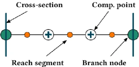
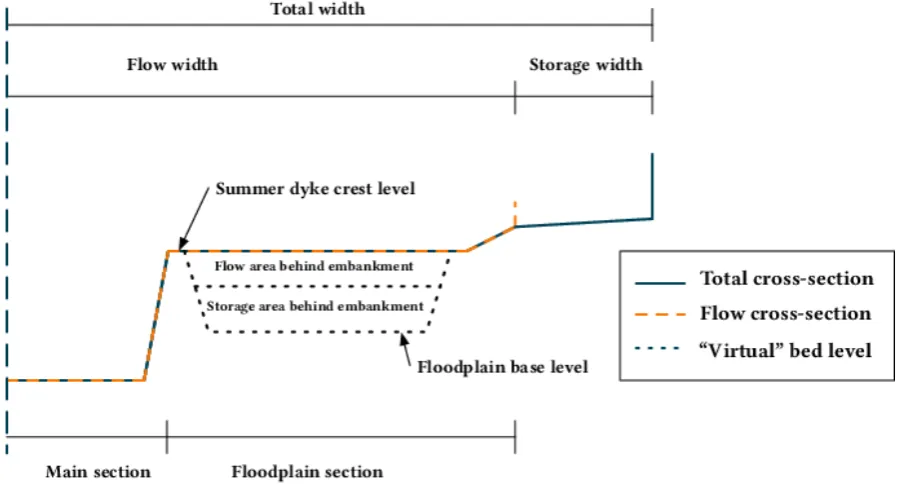
(13) 2.2. SOBEK 3. 6. is created through which water flow is simulated. The network is a collection of nodes connected by lines. Information in 2D, as well as 2D phenomena cannot be included in 1D models. Figure 2.4 shows what the simple 2D model in fig. 2.1 would look like in 1D. To simulate the flow through the network, cross-sections are used to represent the topography. Roughness values can be defined anywhere on the network.. Figure 2.4: Example of a simple SOBEK model with two cross-sections defined at the outer nodes. The small circles are computational points.. SOBEK, named after the ancient Egyptian crocodile river god, is an integrated software package for river, urban and rural management. SOBEK 3 is the latest version of that package and includes seven modules. The module that is of interest here is the 1D flow module, used for simulation of one-dimensional river flow. As with other 1D hydraulic models, SOBEK requires a network with predefined flow paths. In fig. 2.5 a single branch of such a network in SOBEK is illustrated with the corresponding terminology. A branch in the 1D model is a collection of two nodes connected by a line. Along this branch cross-sections can be defined that determine the slope and topography. Between the nodes at the end of the branch, computational grid nodes are inserted on which the waterlevels are resolved. The shape of the cross-section at such nodes is interpolated between the two defined cross-sections.. Figure 2.5: Illustration of a SOBEK network with definitions.. SOBEK uses a staggered grid for computations, meaning that waterlevels and velocities are resolved at different points. The waterlevel is computed on the grid nodes, while the velocities are computed at reach segments, halfway between nodes. This causes the same issues at the boundaries as with Flexible Mesh, where a non existing node or velocity point outside of the domain is necessary to compute the waterlevel at the boundary. SOBEK however solves this issue in a different way than Flexible Mesh and foregoes the usage of ghost cells. Instead, as is illustrated in fig. 2.6, the outer nodes of a branch function as ghost nodes. The discharge from the discharge boundary is imposed on the next velocity point in the branch, and the waterlevel is imposed on the last node. The cross-sections that are used contain a number of elements (fig. 2.7). The total crosssection is the most outer shape, containing both the flow and storage. Another cross-section determines the what part of the cross-section contains flow. The difference between both determines the storage. The flow cross-section is divided into a main section and one or two floodplain sections. Every section has its own roughness values..

(14) 2.3. FM2PROF. 7. Figure 2.6: SOBEK boundary conditions.. It is possible to use embankments, referred to as summer dykes in SOBEK. The area behind the summer dyke is then added “virtually” to the cross-section and divided into flow and storage area.. Figure 2.7: Illustration of the elements of a symmetric SOBEK cross-section.. 2.3. FM2PROF. FM2PROF is a method used for generating 1D hydraulic river models from 2D model results. It uses 2D flow model output to construct the 1D model. By dividing the river into controlvolumes (as illustrated in fig. 2.8) and aggregating results for each control-volume in time, it is possible to construct cross-section geometry and the corresponding roughness values for the main channel and the floodplain. An illustrated explanation to this process is given later in the section, and a quick illustrated overview can be found in appendix A. Features such as embankments however cannot be accounted for in the cross-section, due.

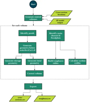
(15) 2.3. FM2PROF. 8. to the fact that inhomogeneous waterlevels cannot be computed in 1D. To account for this the water volume in the cross-section is corrected with a logistic function.. Figure 2.8: Control volume illustration for FM2PROF (adapted from Berends et al., 2016). 2.3.1. Assumptions. A number of assumptions have been made for the method to work. First, it is assumed that in every control volume only one main channel is present; the rest is identified as a single floodplain. It is further assumed that all ponds are filled with water at the start of the simulation in the 2D model output and that the waterlevel in the ponds does not fluctuate with the waterlevel in the main channel. This effectively means that all ponds are detached from the main channel. The output of the 2D model should conform to a few requirements. The waterlevels in the river should rise slowly, monotonically and uniformly over the whole river length. Its output should include waterlevels at flow nodes and Chézy roughness values and flow velocities at flow links. To construct the control-volumes, cross-section locations must be provided. The shape of the control volume for each cross-section is then determined with the nearest-neighbour algorithm.. 2.3.2. Construction. A simplified flow-diagram of the construction procedure in FM2PROF is given in fig. 2.9. A detailed diagram can be found in fig. A.1 in the appendix. The first step is to generate the control volumes. This is done by using the nearest neighbour algorithm for every cell in the 2D model output. Every cell is connected to the closest cross-section point. This partitions the 2D model into control volumes. For every control volume the cross-sections and roughness values are constructed. This is done in a number of steps, which are simplified in fig. 2.9. First ponds are identified and their cells masked. Ponds are only included in calculating the cross-section widths once their waterlevel starts to rise. Then the 2D output is used to generate the cross-section profiles..

(16) 2.3. FM2PROF. 9. Figure 2.9: A simplified flow diagram of the FM2PROF method.. The method with which this happens warrants some further explanation, which is given in section 2.3.3. When generating the cross-section profile, every waterlevel possible in that profile must be present in the 2D model output. This is not the case when the simulation starts with a wet bed. When this occurs, the cross-section profile beneath the initial waterlevel is generated by artificially lowering the waterlevel in FM2PROF, and calculating which cells in the 2D model would have been wet. This process is further covered under improvements in section 3.2. After the full cross-section profile has been generated, the parameters of the volume correction function are determined. Parallel to the generation of the cross-section profile, the roughness section widths and the corresponding values are calculated. Every control volume gives one cross-section and roughness table (for the main channel and floodplain). These cross-sections and roughnesses are then exported in a format that is recognisable to SOBEK 3.. 2.3.3. Cross-sections. Cross-sections are a requirement for 1D hydraulic models. Constructing cross-sections involves some way of simplifying 2D topography into cross-section profiles. Often such cross-sections are “cut” from the available topological data, creating a local line represen-.

(17) 2.3. FM2PROF. 10. tation. Castellarin et al. (2009) mention that there are multiple ways to cut, but in every method a representation is created that does not include topological features not on the line. Furthermore, some features cannot be included by cutting, such as ponds or embankments, and the cross-section must be retroactively corrected for them. FM2PROF makes use of another approach for constructing the cross-sections. When generating surrogates of 2D hydraulic river models, more data is readily available than just the topography or field measurements. Because 2D model output is analysed, it is possible to get the flow conditions at every point in the domain and at each time step. FM2PROF makes use of this, and instead of cutting cross-sections it uses aggregation to construct them. By dividing the river into control-volumes (fig. 2.8) and lumping the 2D flow information inside of them, we attempt to generate cross-sections. The cross-sections are representative for the flow conditions and the topography, but may not resemble the actual topography in the control volume. To construct the cross-sections, the waterlevel in the main channel at the cross-section point is used as a point of reference. For every such waterlevel, the cross-section width is calculated. It is assumed that the waterlevel is the (vertical) z-coordinate for the calculated cross-section width. Doing this for every waterlevel allows to construct a cross-section profile, as illustrated in fig. 2.10. The cross-section width is calculated by summing the area of all wet cells for that waterlevel, and dividing it by the cross-section length.. Figure 2.10: Cross-section from a 2D model with a rising waterlevel. The H stands for the waterlevel in the middle of the main channel, and the black rectangles are embankments. W is the calculated cross-section width for waterlevel H.. 2.3.4. Identification. For the correct generation of roughness values and the correct reproduction of the main channel and floodplain section width, it is necessary to identify which cells belong to the main channel and which belong to the the floodplain. For the section widths, it is necessary to differentiate the main channel from the floodplain. This is done by assuming that main channel is smoother than the floodplains. For the last timestep in the simulation, when the channel is full, a roughness “cutoff” value is determined by variance minimisation of all roughness values in the control volume (eq. (2.1)). As Chézy values are used for the roughness, this means that higher values belong to the main channel. Flow links with a value higher than the cutoff are therefore attributed to the main channel, and the other flow links are attributed to the floodplain. It is then possible to find which.

(18) 2.3. FM2PROF. 11. cells belong to the main channel and which belong to the floodplains. Summing the area and dividing by the length of the control volume (the same procedure as determining the cross-section widths for every waterlevel) gives the widths of the roughness sections. f (z i ) = [max(V ar (z > z i ),V ar (z ≤ z i ))]. (2.1). where f (z i ) is the function that is minimised, z is an array of Chézy roughness values and z i is the cutoff value. Var() is the variance function and max() extracts the maximum values element-wise.. 2.3.5. Volume correction. The generated 1D cross-sections cannot reproduce the 2D water balance in a control volume if the waterlevels are inhomogeneous. A clear example of this are embankments, which cannot be included in the cross-section geometry. When embankments are present and they start to flood, the volume will increase in the 2D model, but the waterlevel in the main channel will not. In a 1D cross-section, this cannot be accounted for with geometry alone. In such a case FM2PROF will generate a geometry where the floodplain starts at the peak of the embankment, due to the cross-section widths being generated for waterlevels in the main channel. Therefore the volume in the 1D cross-section will be smaller than in 2D. The disparity in water volume between the generated cross-section and the 2D control volume is corrected with a two parameter logistic function. The parameters are calculated through error minimisation between the 1D and 2D volumes. The equation is: C (h k ) = Ξ(1 + e l og (δ)τ. −1. (h k −(γ+ τ2 )) −1. ). (2.2). where Ξ is the required volume correction [m3 ], τ is the transition height over which the volume become available to the 1D model [m], δ is an accuracy parameter [-] and γ is the water level at which the extra volume becomes available [m] The parameters that are calculated are the extra released volume Ξ and the accuracy parameter δ. The transition height τ is a parameter that can potentially be adjusted as well, but as SOBEK 3 does not yet provide the ability to adjust this parameter on a per cross-section basis, so it is kept at the default value 0.5m.. 2.3.6. Storage and ponds. Not all water in a river reach will be flowing. Features such as groynes can interrupt water flow, creating storage and pushing up the waterlevel. Other times the floodplain includes an area that is deep and filled with water, also known as a pond. If a pond is detached from the main channel its waterlevel does not fluctuate until the floodplain floods, but that is not necessarily the case as a pond may be connected to the main channel. It is important to identify storage and ponds in a control volume for a correct reconstruction of the cross-section profile. Storage sections are recreated by identifying flowing cells in the 2D model, and constructing a cross-section for flow. Subtracting the flow cross-section from the total cross-section gives what is known in sobek as the storage area (see fig. 2.7 and section 2.2 for cross-section definitions). Which cells contain flow, and which contain stored volume is determined with two parameters: an absolute and a relative one. The absolute parameter checks whether the velocity in a cell exceeds an absolute value. If it does, the cell.

(19) 2.3. FM2PROF. 12. contains flow. The relative parameters is for comparing the velocity in a cell to the average velocity in the control-volume for a timestep. If the velocity in a cell exceeds the average velocity in a control volume times the relative parameter, the cell contains flow. This is done for every timestep in the 2D model output, allowing the generation of flow cross-section. Ponds are deep and are filled with water at any time in the simulation. Not excluding these wet cells in the 2D model would overestimate the cross-section profile width until the waterlevel is high enough for the pond to flood. Ponds are identified by marking cells that are wet at the start of the model run and whose waterlevel does not rise for a number of timesteps. This value was set to 10 timesteps of 1 hour each. The number of steps to use depends on the 2D model initial conditions and the interval for each step. The cells are then excluded from the calculation until the point that the waterlevel in a those cells does start to rise. Ponds attached to the main channel are assumed to be part of the main channel with this approach, because their waterlevel will fluctuate with the waterlevel in the main channel.. 2.3.7. Parameters. A number of parameters are used during the construction of the cross-section geometry. The parameters have been tabulated in table 2.1. Table 2.1: FM2PROF parameters. #. Parameter. Default. Unit. Description. 1 2 3 4 5 6 7 8. num_css_points abs_vel_treshold rel_vel_threshold delta gamma css_distance min_depth_storage step_ponds. 20 0.01 0.03 n.a. n.a. 500 0.02 10. m/s m m m -. Number of points in final, simplified cross-section Absolute velocity threshold for determining cells with flow Relative velocity threslhold for determining cells with flow Volume correction accuracy parameter Water level at which extra volume becomes available Distance between cross-sections Minimum depth for the storage identification Number of timesteps for pond identification.

(20) Chapter 3 Method The objective of this thesis is to construct 1D hydraulic river models from 2D model results. This has been done by expanding upon the proposed FM2PROF method that works by aggregating 2D model results. This section covers the method used in answering the research questions (RQ) and achieving the objective. First a validation framework was constructed (RQ1). The framework consists of two parts: verification and validation. The FM2PROF output (cross-sections, roughness values, volumes) is verified to be either expected or satisfactory and the 1D model results are validated. For both steps multiple test cases are constructed. Idealised test cases were used to verify that FM2PROF generates the expected output for different possible elements in a river. The 1D models are then constructed using that output and their results validated against the 2D model results. Last, a model of the river Waal was chosen as a final, complex test case that includes all features that were verified and validated before with the idealised cases. Second, improvements to the FM2PROF method were implemented (RQ2). Using the idealised test cases from the validation framework (RQ1), FM2PROF output and 1D model results were used to find points of improvement. Where the results were not as hypothesised, improvements were implemented and the 1D models generated again. This process was repeated until results were satisfactory. The last step was to generate 1D models using FM2PROF for each test case and to validate the 1D model output (RQ3).. 3.1. Research question 1: Validation. It is important to promote confidence in the methods that are used. The first part of creating confidence in the FM2PROF method is to confirm that the output of the method is as we expect for different conditions. Understanding where it is not and why it is different is just as important. To achieve this, verification of the FM2PROF output was carried out, after which the constructed 1D model results were be validated. Validating a surrogate, like validating any model, can be a challenging task. Even the meaning of the term and the goal of the procedure is a topic of discussion in the scientific community (Rykiel, 1996). For the validation framework of the surrogate the definition of operational validation was adopted. This means that the model was deemed satisfactory if it possessed an accuracy consistent with the intended application of the model under specified conditions. This is a practical definition that is suitable for engineering purposes. 13.

(21) 3.1. Research question 1: Validation. 14. The purpose of the surrogate was taken from the objective, namely to emulate 2D model results. The operational context that defines the specified conditions was taken as operational forecasting and long term prediction of hydraulic river conditions. The geographical context determines what conditions must be included in the framework to validate the model for its operational context. Since the intended use of the surrogate is initially limited to the country of the Netherlands, flow conditions limited to that geography were taken into account. This means that conditions such as critical flow or complex flow in braiding rivers were not considered. This section will cover the details of the validation framework that was used. First an overview of the steps in the framework is given, after which the topic of calibration will be touched upon. The choice of indicators is then covered, after which the verification and validation steps are expanded upon.. 3.1.1. Overview. First the output of FM2PROF was verified. Since such an effort is impossible for complex cases where the aggregation makes a direct comparison impossible, this was done for idealised cases first. Simple, idealised cases were used to verify the FM2PROF output for different features (e.g. embankments) separately. The goal was to split what the surrogate should be able to emulate into small parts and to verify that separately. A total of seven idealised cases were used (described later in the chapter). A 2D model of the river Waal was taken as the complex case to validate a combination of all the features that were tested for in the idealised cases. FM2PROF output for the idealised cases was verified by comparing the generated output to the extracted results from the 2D model. Any direct comparison was impossible for the complex case, so the verification for that was carried out by judging the output in broad lines, so whether the output resembles what is found in the control volume in the 2D model. After that 1D surrogates were constructed for each case and their output was validated. This was done for both monotonically rising conditions as well as for a discharge wave. The validation was carried out by comparing waterlevel values in the main channel in the 2D models to the waterlevels in the 1D model results.. Figure 3.1: Example of a monotonically rising discharge boundary condition. Figure 3.2: The discharge wave used for idealistic cases..

(22) 3.1. Research question 1: Validation. 3.1.2. 15. Calibration. A challenge in validating surrogates lies in deciding on a rigorous method (Fernández-Godino et al., 2016). What values to compare and how is an important question. Relevant to this is whether to calibrate the 1D model before carrying out the validation method. The 1D models are validated in an uncalibrated state, with the roughness values that come directly from FM2PROF. This is because with calibration it is much more difficult to state whether it is the produced surrogate that is correct, or whether it is deficient but has been calibrated to a satisfactory accuracy. As the purpose of the constructed 1D model is to emulate the model results, it is not the accuracy after calibration that is important to judge, but the overall surrogate behaviour. Analysing results of the uncalibrated model gives a better indication of how well the emulation is achieved. The used 2D models for the generation of the surrogates are not calibrated either. Since a direct comparison between model and surrogate is used, any state of the 2D model could be used. Importance was assigned to whether the surrogate would emulate 2D model results, irrespective of whether the 2D model was calibrated. Using a calibrated 2D model would change the roughness values in the main channel of the 2D model, and FM2PROF would then use the new values in the aggregation.. 3.1.3. Indicators. Objective indicators are often used when validating models. Because the purpose of the 1D model was emulation of the 2D model results and it was decided not to calibrate the 1D model, using objective indicators was not appropriate. For the validation the performance of the surrogate model was not defined as a quantitative measure of accuracy, but rather as the general emulation of the 2D model behaviour. Therefore the surrogate was deemed satisfactory (or not) by comparing the model behaviour between the 1D surrogate and the 2D model instead of using absolute performance measures.. 3.1.4. Verification. A number of indicators were used to judge the FM2PROF output. The verification of a case was considered satisfactory if: a) cross-section geometries match the expected shape; b) the main channel and floodplain section widths correspond between the cross-section and the 2D model; c) the averaged roughness values correspond to the expected values from the 2D model; d) the corrected total water volume error is less than 5%. All the indicators will be covered one by one. Cross-section geometry The first indicator was cross-section geometry. This includes the total cross-section geometry and if present, also storage areas. The generated cross-section geometry was compared.

(23) 3.1. Research question 1: Validation. 16. visually to the shape that was used to construct the idealised test case. For the complex case only general observations can be made about the overal shape, storage areas and section widths, as the topology is aggregated into cross-sections that may not resemble reality. An example of such a direct comparison for an idealised test case is illustrated in fig. 3.3. The generated cross-sections are symmetric, therefore plotting one half is sufficient. On the y-axis the waterlevel for which the cross-section width has been determined is plotted. The “original” geometry, taken from the uniform 2D model is compared to the generated geometry.. Figure 3.3: Cross-section geometry comparison example taken from a test-case for a compound channel.. Storage area, if present, is compared from the generated SOBEK cross-section (fig. 3.4). The storage area is shown in the symmetric cross-section, with the total storage area in the bottom right corner..

(24) 3.1. Research question 1: Validation. 17. Figure 3.4: Cross-section from SOBEK, with the total cross-section and storage areas plotted.. Roughness section widths The roughness section widths for idealised cases are known beforehand. The generated main channel and floodplain widths are then compared to them in a table form. For uniform channels only one value exists for the main channel and one for the floodplain. Example: Table 3.1: Comparison of roughness widths. Roughness section. Section width [m]. Correct section width [m]. Main channel Floodplain. 50.0 100.0. 50.0 100.0. Roughness tables The second verification indicator is bedlevel roughness values. FM2PROF aggregates all roughness values over what it has identified as the main channel and then over the floodplain. This is done for every waterlevel available in the 2D model output, so a figure such as fig. 3.5 can be created. The averaged roughness values for every waterlevel are compared to the expected roughness values. The expected values are taken from the 2D model as manning values and converted to their Chézy equivalents according to eq. (3.1) (Deltares Systems, 2017a). C=. h 1/6 n. (3.1).

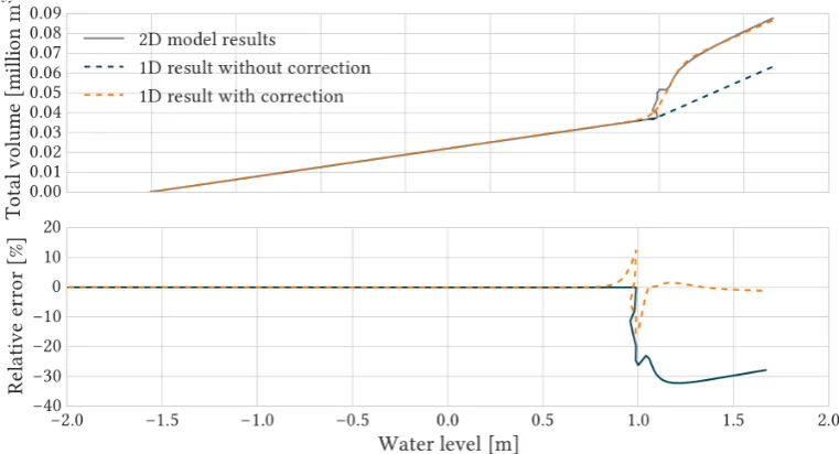
(25) 3.1. Research question 1: Validation. 18. Figure 3.5: Cross-section roughness comparison example taken from a test-case for a compound channel. Two curves can be seen, one for the main channel with higher roughness values, and one for the floodplain.. Volume - waterlevel plots The last indicator used for verification is a volume - waterlevel plot. The volume in the cross-section as well as the 2D control-volume is plotted for every waterlevel. The volume in the cross-section after the correction is shown too. The relative error for every waterlevel is shown underneath. An example from a control-volume with an embankment is shown in fig. 3.6.. Figure 3.6: Watervolume comparison example taken from a test-case with an embankment..

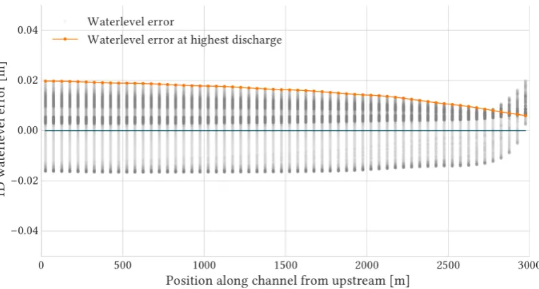
(26) 3.2. Research question 2: Improvements. 3.1.5. 19. Validation. Visual comparison was used when comparing the waterlevels in the 1D and 2D models. Due to the difference in dimensionality, in 2D the waterlevels in the main channel were used taken at the cross-section points used to generate the control volumes. Thus the waterlevels in 1D were compared to waterlevels in the main channel in 2D. For every time step the waterlevel error at every computational point along the length of the 1D model was plotted. This results in a dotty plot with every available waterlevel value being compared between the 1D and 2D model. The points at the timestep with the highest discharge at the upstream boundary are connected and highlighted to give insight into the slope of the water surface at that point. An example is given in fig. 3.7. The grey lines are collections of grey dots, which are the waterlevels for every timestep and every computational point in SOBEK. Darker sections show that more waterlevel errors were found of that magnitude.. Figure 3.7: Waterlevel error plot example.. Assigning a quantitative threshold that determines whether the model results pass validation is not trivial. Mashriqui et al. (2014) accept maximum errors of up to 0.4m with a mean of 0.25m for extreme events. No such events are used for validation here, instead a single discharge wave is applied. The acceptable mean error from Mashriqui et al. (2014) was used, making the threshold for determining whether the surrogate passes validation 0.25m.. 3.2. Research question 2: Improvements. The process of verification and validation of the FM2PROF method for every test case was iterative in nature. First the output was analysed, and if deemed not satisfactory improvements would be made and the results generated and analysed again. This process is illustrated in figure 3.8. As a result of this approach a number of errors were found and subsequently improvements were added to the method to improve the results..

(27) 3.3. Research question 3: Test cases. 20. Figure 3.8: Method diagram for a single test case. 3.3. Research question 3: Test cases. A total of eight test cases was created. Seven idealised ones, and one complex case. Every idealised case is used to validate a different aspect. The test cases are ordered from simple to more complex, with the last case being the river Waal model. All idealised cases are straight channels of 3000m length. The slope is always 3.33 · 10−4 , making the total drop in elevation over the whole length 1m (illustrated in fig. 3.9). The total width is 150m, and if a main channel is present, it is 50m wide. A top view of the test cases is shown in fig. 3.10. The only exception to these dimensions is case 3 with the triangular grid, due to the ready availability of the model in other dimensions.. Figure 3.9: Side view for idealised test cases. Figure 3.10: Top view for idealised test cases. Every test case was validated using two discharge boundary conditions. One monotonically rising discharge series and a discharge wave. A selection of test cases was made based upon the features that can be encountered in 2D models. These were: a) topography b) main channel and floodplain c) storage flow d) embankments e) ponds.

(28) 3.3. Research question 3: Test cases. 21. Furthermore, FM2PROF should work for rectangular as well as triangular grid-cells in the 2D model. The shape of the cell impacts how the topography is defined and how features such as embankments are positioned. 2D models can contain one or both types of cells. The selection of test cases was therefore as follows: 1. a rectangular channel; 2. a compound channel; 3. a compound channel with a triangular grid; 4. a three-stage compound channel; 5. a compound channel with storage added to the floodplains; 6. a compound channel with embankments; 7. a compound channel with a pond; 8. the river Waal;. 3.3.1. Case 1 - rectangular channel. The first case is a uniform rectangular channel. There is no main channel or floodplain, and only one roughness value has been used. The cross-section shape can be seen in fig. 3.11.. Figure 3.11: Cross-section for case 1.. The case is meant to test for the following: • Construction of the cross-section profile for simple geometry. • Reconstruction of one roughness curve. • Reconstruction of one roughness section width.. 3.3.2. Case 2 - compound channel. The second case is a uniform compound channel. The main channel and floodplain have their own roughness values and the geometry is more complex when compared to the first case. The cross-section shape is as seen in fig. 3.12..

(29) 3.3. Research question 3: Test cases. 22. Figure 3.12: Cross-section for case 2.. The case is meant to test for the following: • Construction of the cross-section profile for more complex geometry, specifically the transition from main channel to floodplain. • Reconstruction of the main channel and floodplain section widths. • Reconstruction of two roughness curves.. 3.3.3. Case 3 - triangular grid. The third case is very similar to the second case, but the rectangular cells have been replaced with triangular ones. The dimensions of the model are different:. Figure 3.13: Cross-section for case 3.. Expected results. Figure 3.14: 2D model mesh for case 3 at the upstream boundary.. The case is meant to test for the following:. • Construction of the cross-section profile for a mesh with triangular cells. • Reconstruction of the main channel and floodplain section widths for a mesh with triangular cells. • Reconstruction of the roughness curves for a mesh with triangular cells.. 3.3.4. Case 4 - three-stage compound channel. The fourth case is a more complex version of the compound channel, namely a three-stage compound channel. The main channel has the same dimensions, but the floodplain is now separated into two parts with a different elevation..

(30) 3.3. Research question 3: Test cases. 23. Figure 3.15: Cross-section for case 4.. The case is meant to test for the following: • Construction of the cross-section profile for more complex geometry, specifically more detailed floodplains. • Reconstruction of two roughness curves from non-homogeneous floodplain. It is expected that the roughness values for the floodplain will be an average of the two original curves (one for each stage in the floodplain).. 3.3.5. Case 5 - storage. The fifth case is meant to check whether storage is correctly identified by FM2PROF. The topography is the same in case 2: a compound channel. Thin dams have been added to the floodplain in a control volume to create a storage area (illustrated in fig. 3.16). Thin dams are infinitely thin and infinitely high walls that can be added to Flexible Mesh models. By adding thin dams to each cell in the perpendicular direction of the flow, water can enter the cell but doesn’t flow to the neighbouring cells.. Figure 3.16: Top down view .. The case is meant to test for the following: • Construction of flow cross-sections, and by extension... • the generation of storage sections in the total cross-section (total cross-section minus flow cross-section gives storage area in SOBEK, see section 2.2). It is expected that the storage will be slightly underestimated due to velocities in cells near the main channel being higher (and therefore possibly classified as not storage). Furthermore, the waterlevels upstream of the thin dams are expected to be underestimated in the 1D model, due to the build up of water that is captured in the 2D model but which is not present in the 1D model because only storage is added, not a barrier such as a thin dam..

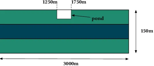
(31) 3.3. Research question 3: Test cases. 3.3.6. 24. Case 6 - embankments. For case 6 the volume correction function is tested by including embankments in the 2D model. The embankments are added along the main channel and are 1m high, as can be seen in fig. 3.17.. Figure 3.17: Cross-section for case 6.. The case is meant to test for the following: • A correct adjustment of the volume-waterlevel curve.. 3.3.7. Case 7 - ponds. For the test case with the pond a compound channel topography was taken as the basis. The 2D mesh was made finer to allow the addition of a pond to the floodplains. The pond was added to the middle control volume on one of the floodplain banks (between 1250m and 1750m). The pond was 10m deep.. Figure 3.18: Illustration as a top down view for the 2D model, showing the location of the pond.. The case is meant to test for the following: • Construction of the cross-section profile, specifically identifying the pond and masking it out from the cross-section generation until the pond is flooded.. 3.3.8. Case 8 - Waal. The final case is for a 2D model of the river Waal. A short summary of the study area, cited from Warmink et al. (2013, p. 303):.

(32) 3.3. Research question 3: Test cases. 25. River Waal is the largest distributary of River Rhine in the Netherlands .... With an annual average discharge of 2250m3 /s, River Rhine bifurcates into the Pannerdensch Kanaal and River Waal, 20 km after entering the Netherlands. River Waal has a length of 93 km, and roughly 2/3 of the total discharge in the Rhine is directed towards the Waal. The width of the main channel of River Waal between the groynes is 280 m on average (Yossef, 2005), and the cross-sectional width between the embankments varies between 0.5 km and 2.6 km (Straatsma and Huthoff, 2011). The total embanked area of River Waal in the Netherlands is about 184km2 , including the main channel, the groyne fields and the flood plain areas. The flood plain area and groyne fieldstogether make up 73% of the total embanked area. The landcover of the flood plains is dominated by meadows, but recent nature rehabilitation has led to increased areas with herbaceous vegetation, shrubs and forest (Straatsma and Huthoff, 2011). The Waal has an average water level gradientof 0.11 m/km (Middelkoop and van Haselen, 1999). The dimensions of the 2D Waal model are many factors higher than the idealised cases. Ponds, embankments, groynes, complex topography and gradual changes in bed roughness are all present. A control volume from the 2D model was used for the verification step, marked in fig. 3.19. The upstream boundary condition is located at Pannerdensche Kop, and the model ends at Hardinxveld. The 2D model simulation that is used to construct the surrogate is run with a nearly full main channel as the initial conditions. This is due to the difficulty with stability for running the model with dry initial conditions.. Figure 3.19: A part of the grid of the 2D FM Waal model with the bedlevels. The white rectangle marks the approximate area of the control volume used for the verification step.. It is expected that the storage area will be underestimated due to the presence of groynes in the Waal main channel, which are not captured because no 2D model results are available for low waterdepths.. 3.3.9. FM2PROF setup. The FM2PROF input consists of the 2D model results and a cross-section location file (section 2.3). The waterlevel in the 2D model results should rise monotonically and uniformly. For the idealistic cases the boundary conditions are calculated to fulfil this condition. For the complex case an approximation for those is used, with long simulation times and a slow rate.

(33) 3.3. Research question 3: Test cases. 26. of increase of the discharge at the boundary. For the idealised cases a rate of 10cm per day is used for the calculations, so that the output has a high enough resolution to generate the sharp edges in the cross-section profiles..

(34) Chapter 4 Results The results are presented in the order of the research questions. First the used validation framework is summarised (RQ1), then the improvements are presented (RQ2), and finally results of the verification and validation for test cases are shown (RQ3).. 4.1. Research question 1: Validation. The validation framework that was constructed consists of two steps: verification and validation. To breed confidence in the FM2PROF method its output was verified. This is done by comparing the cross-section profiles, generated roughness values and the watervolume with the 2D model. The 1D model that is generated with the FM2PROF output is then validated by comparing its waterlevels for all timesteps and all computational points with the 2D model results. Both the verification and validation is carried out for test cases that are constructed to test whether 2D model features are correctly reproduced by FM2PROF. A total of eight test cases are used for the verification and validation. Seven are idealised with uniform profiles, while the last is a complex 2D model of the river Waal. For every test case two discharge boundaries are used: a monotonically rising discharge and a discharge wave. For both situations the waterlevel errors are plotted and analysed.. 4.2. Research question 2: Improvements. As described in the method (section 3.2) a number of potential improvements were identified and consequently implemented.. 4.2.1. Wet initial conditions. The original implementation of FM2PROF required the bed in the 2D model to be dry at the beginning of the simulation. Filling the bed slowly and monotonically allows the calculation of the cross-section width at every waterlevel by identifying wet cells and averaging their area. It is however not always possible to start a complex model from a completely dry bed. Another problem that occurs when starting from a dry bed is that cells become wet gradually, leading to errors in cross-section geometry. At the initial timesteps the cross-section width will be underestimated simply because not all cells have become wet. By the time the 27.

(35) 4.2. Research question 2: Improvements. 28. main channel has filled up, the waterlevel has risen, resulting in an error in the generated geometry.Figure 4.1 illustrates the error. Note that the same issue occurs when the floodplain starts to flood, for the same reasons. Finally, cells may be misassigned as storage cells due to the low flow velocities during the initial filling up of the main channel.. Figure 4.1: Illustration of the cross-section geometry error that occurs during the stages when a channel section is getting wet.. To solve this issue the method has been modified to allow the simulation to start from a wet bed. This is done by “virtually” lowering the water level in the model results and retroactively calculating which cells should be wet at that water level. The water depth is calculated at the initial time step (t=0). The waterlevel is then lowered step by step until the depth becomes zero. For every step, wet cells are identified and aggregated. It is assumed that at t=0 only the main channel is wet.. 4.2.2. Roughness values on flow links. The original implementation used roughness values at cell centers to construct roughness tables. Due to the staggered grid in Flexible Mesh, roughness values are defined on cell edges, and the value in the cell center is the average of the values at all edges. Using average values introduces an error in the identification of the main channel and flood plain width. This is because taking the averages causes FM2PROF to misidentify the cells at transitions between the main channel and the floodplain. This has been solved by calculating directly with the roughness values at the cell edges. The edges are then identified as either belonging to the main channel or the floodplain. It is then possible to assign cells to either the main channel or the floodplain by analysing to what class their cell edges belong. If a cell has two edges belong to one class and two to another, it will be identified as an alluvial cell.. 4.2.3. Storage identification. Storage in a control volume is identified by analysing the velocities and determining whether the water in a cell is flowing, or is stagnant. The difference is determined by using two factors: an absolute velocity threshold and a relative velocity threshold. In practice, this method overestimated the storage in a control volume. When the floodplain is wetting, flow velocities are of a small order. This leads to most floodplain cells being.

(36) 4.3. Research question 3: Test cases. 29. attributed to storage while the water depth in the floodplain is low. This overestimation was countered by applying a water depth mask: by eliminating cells from the calculation with a water depth below a certain threshold. This threshold is defined as a parameter and set to two centimetres. Outliers in 2D flow velocities may also lead to overestimation of storage area. Both the geometry and numerical computations introduce errors into the results: for very short timespans, in the order of one timestep, flow velocities can become large enough to identify the cell as flowing even when it is part of storage. These small errors propagate due to the cross-section geometry simplification algorithm being sensitive to outliers. The issue was solved by smoothing out the outliers with a rolling average in time for all velocity values.. 4.2.4. Pond identification. Not excluding wet cells of ponds in the 2D model overestimates the cross-section profile width until the waterlevel is high enough for the pond to flood. However the initial method would include them and therefore overestimate the cross-section widths. Pond identification has been added to avoid the overestimation. Ponds are identified by marking cells that are wet at the start of the model run and whose waterlevel does not rise for a number of timesteps. The cells are then excluded from the calculation until the point that the waterlevel in a those cells does start to rise. The assumption that the waterlevel does not rise or fall until the floodplain floods identifies ponds that are detached from the main channel. If a pond is attached, the cells will simply be taken as being part of the main channel and classified as storage if the flow velocity is low.. 4.3. Research question 3: Test cases. The results of the verification and validation for all test cases is given here. For the verification, where possible, the cross-section profiles between 1D and 2D are compared. The roughness values for each waterlevel are compared to analytic calculations if those can be made, and the volumes in control volumes are compared to volumes in cross-sections in 1D. Where necessary, pond identification maps and visualisation of flow link categorisation is used to further understand the verification results. For the validation the waterlevel differences between 1D and 2D are plotted for every calculation point in the 1D model. This is done for all timesteps.. 4.3.1. Case 1 - rectangular channel. The cross-section profile is reconstructed accurately and the roughness table contains a single Chézy curve corresponding to the correct manning value of 0.03. The roughness section width for the main channel is 150 metres. The volume in the 1D model is overestimated, and the volume correction function attempts to rectify the difference by adding “negative” extra volume. Negative values for the correction are not applied in the 1D model, and in such cases the volume correction is simply skipped by SOBEK..

(37) 4.3. Research question 3: Test cases. (a) Comparison between the generated and the original cross-section.. 30. (b) Comparison between the generated and the original roughness values for the cross-section.. (c) Comparison of the volume in the cross-section to 2D model output. Figure 4.2: Verification of FM2PROF output for case 1.. Table 4.1: Generated roughness section widths for case 1. Roughness section. Section width [m]. Correct section width [m]. Main channel. 150.0. 150.0. Validation The waterlevel errors are in the order of centimetres, with a maximum error of 4 centimetres underestimation. The biggest deviation occurs for the peak discharge during a wave. The waterlevel slope is not correctly emulated, and the waterlevel is both over- and underestimated..

(38) 4.3. Research question 3: Test cases. 31. (a) Waterlevel errors for a monotonically rising discharge.. (b) Waterlevel errors for a discharge wave. Figure 4.3: Validation for case 1: waterlevel errors between 1D and 2D for all locations along the channel and all timesteps in the simulation.. 4.3.2. Case 2 - compound channel. The cross-section profile is reconstructed accurately. However, an error occurs at the sharp corner in the transition from the main channel to the floodplain. This is due to the fact that the floodplain does not flood instantly in the 2D model. In 1D however, the transition from main channel to floodplain is instantaneous, and therefore a peak in the volume error between 1D and 2D is expected the moment the floodplain floods. For the roughness table, two Chézy curves are be visible, one for the main channel (manning of 0.03) and one for the floodplain (manning of 0.07). The roughness section widths are also correct..

(39) 4.3. Research question 3: Test cases. (a) Comparison between the generated and the original cross-section.. 32. (b) Comparison between the generated and the original roughness values for the cross-section.. (c) Comparison of the volume in the cross-section to 2D model output. Figure 4.4: Verification of FM2PROF output for case 2. Table 4.2: Generated roughness section widths for case 2. Roughness section. Section width [m]. Correct section width [m]. Main channel Floodplain. 50.0 100.0. 50.0 100.0. Validation The waterlevel errors for the compound test case are consistent. The slope is better approximated than with the rectangular test case, and the error is in the order 5 centimetres. For both the wave and a monotonically rising discharge the waterlevel is underestimated for the peak discharge. Because the 2D model simulates internal friction in the flow as well (something that does not happen in 1D), higher waterlevels in 2D are to be expected in uncalibrated comparisons..

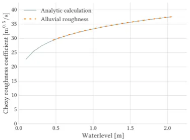
(40) 4.3. Research question 3: Test cases. 33. (a) Waterlevel errors for a monotonically rising discharge.. (b) Waterlevel errors for a discharge wave. Figure 4.5: Validation for case 2: waterlevel errors between 1D and 2D for all locations along the channel and all timesteps in the simulation.. 4.3.3. Case 3 - triangular grid. The cross-section profiles are accurately reproduced. The error in roughness values for the floodplain is due to an error in the implementation of FM2PROF. The floodplain in the 2D model output has the correct roughness values, and both the main channel as well as the.

(41) 4.3. Research question 3: Test cases. 34. floodplain is identified correctly.. (a) Comparison between the generated and the original cross-section.. (b) Comparison between the generated and the original roughness values for the cross-section.. (c) Comparison of the volume in the cross-section to 2D model output. Figure 4.6: Verification of FM2PROF output for case 3.. 4.3.4. Case 4 - three-stage compound channel. The cross-section profile is reconstructed accurately. The addition of another elevation in the floodplain causes the roughness values to deviate from the analytical calculations. The method assumes that the floodplain contains one Chézy roughness curve, but that is no longer the case. The difference in elevation gives two Chézy roughness curves, but since all roughness values are averaged over the floodplain, the roughness curve for the floodplain is the average of the two separate curves..

(42) 4.3. Research question 3: Test cases. (a) Comparison between the generated and the original cross-section.. 35. (b) Comparison between the generated and the original roughness values for the cross-section.. (c) Comparison of the volume in the cross-section to 2D model output. Figure 4.7: Verification of FM2PROF output for case 4.. Table 4.3: Generated roughness section widths for case 4.. Roughness section. Section width [m]. Correct section width [m]. Main channel Floodplain. 50.0 100.0. 50.0 100.0.

(43) 4.3. Research question 3: Test cases. 36. Validation. (a) Waterlevel errors for a monotonically rising discharge.. (b) Waterlevel errors for a discharge wave. Figure 4.8: Validation for case 4: waterlevel errors between 1D and 2D for all locations along the channel and all timesteps in the simulation..

No results found