On The Fly parallel decomposition of strongly connected components

(1)

University of Twente

Master Thesis

On-The-Fly Parallel Decomposition of

Strongly Connected Components

Author:

Vincent Bloemen (s1004611)

Graduation Committee:

Prof. Dr. J.C. van de Pol

Dr. A.W. Laarman

Dr. S.C.C. Blom

(2)

Abstract

(3)

List of Algorithms

1 Union-Find structure . . . 12

2 Depth-first search (recursive) . . . 13

3 Breadth-first search . . . 13

4 Tarjan’s algorithm . . . 15

5 Dijkstra’s algorithm . . . 17

6 Kosaraju-Sharir algorithm . . . 17

7 Purdom’s algorithm . . . 18

8 Gabow’s algorithm . . . 19

9 Forward-Backward algorithm . . . 20

10 OBF algorithm . . . 20

11 Nested depth-first search . . . 22

12 Lowe’s algorithm . . . 23

13 The Suspend procedure in Lowe’s algorithm . . . 24

14 Renault’s algorithm . . . 25

15 Parallelized (abstract) set-based algorithm . . . 28

16 Extended locklessUnion-Findstructure for the naive approach . . . 31

17 A naive parallel SCC algorithm . . . 32

18 TheUF-SCCalgorithm . . . 38

19 TheMakeClaimprocedure forUF-SCC . . . 39

20 ThePickFromListprocedure forUF-SCC . . . 40

21 TheRemoveFromListprocedure forUF-SCC . . . 40

22 TheMergeprocedure forUF-SCC . . . 41

23 The locking mechanism for theMergeprocedure inUF-SCC . . . 41

24 TheMergeListsprocedure for UF-SCC . . . 41

25 Next-Statefunction for randomly generated models. . . 56

26 TheUF-SCCalgorithm . . . 66

27 Specification for theUF-SCCalgorithm . . . 67

(6)

List of Figures

1.1 Example of a graph in which the marked regions represent the SCCs. . . 5

1.2 Visual representation of the topic for this project. . . 6

2.1 Graph traversal vertex ordering for pre-order DFS, pre-order DFS and BFS. . . 14

4.1 Example depicting the advantage of communicating partially discovered SCCs. . . 27

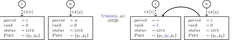
4.2 Example on how a state’sPsetis updated after aUnioncall. . . 30

4.3 Example situation for explaining why a wait procedure is applied in Algorithm 17. . . 33

4.4 Example that shows how a deadlock cycle arises. . . 33

4.5 Example that shows how an incomplete SCC can be markeddead. . . 34

5.1 Illustrative representation for the list mechanism. . . 36

5.2 Illustrative representations of the internal list merge and list removal processes . . . 37

5.3 Representation of the used data structures for theUF-SCCalgorithm. . . 43

6.1 A scatter plot, illustrating statistics for the BEEM models. . . 48

6.2 Speedups of theUF-SCC algorithm compared to its sequential version, fortrivial and non-trivialBEEM models. . . 50

6.3 Speedups of the UF-SCC algorithm on selected models, relative to: its sequential version; Tarjan’s sequential algorithm;Renault’s SCC algorithm. . . 52

6.4 Absolute time usage forTarjan,RenaultandUF-SCCon four BEEM models. . . 53

6.5 Absolute time usage for the UF-SCC algorithm on random models containing 10,000,000 states and a fanout of 5, 10, and 15. . . 56

6.6 Speedups for theUF-SCC algorithm relative to its sequential performance, on specific con-figurations of random graphs. . . 57

6.7 Illustrative representation of the relative dependence relation for methods inUF-SCC64. . . 58

6.8 Relative speedups for the UF-SCC algorithm on non-trivial selected BEEM models, on the weleveld and westervlier machine. . . 60

6.9 Absolute time usage on theat.4BEEM model for a lockless Renault implementation and one where locking is used. . . 61

(7)

Chapter 1

Introduction

In Computer Science, a wide variety of problems can be represented with a (directed) graph structure. A graph describes abstract objects (vertices or states) and the relations that hold between these (edges or

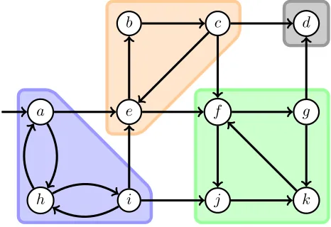
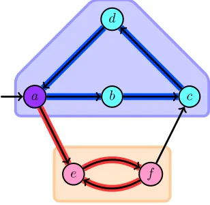
transitions). Consider for instance representing road systems, social networks, or practically any type of process. Graph algorithms are then applied for solving particular problems. One common technique is decomposingstrongly connected components(SCCs); finding sets of vertices for which every vertex can reach each other vertex in the set. Figure 1.1 gives an example of a graph where the marked regions represent distinct SCCs. For instance, verticesb, c, and eare part of the same SCC because these can all reach each other. Applications for SCC decomposition include data- and (social) network analysis, as well as various verification techniques.

b

c

d

a

e

f

g

[image:7.612.193.426.368.528.2]

h

i

j

k

Figure 1.1: Example of a graph in which the marked regions represent the SCCs.

(8)

SCC algorithms

Parallel Sequential

On-the-fly

Our work

(On-the-fly) Offline

Small SCCs Large SCCs

[image:8.612.107.511.86.285.2]

Graphs

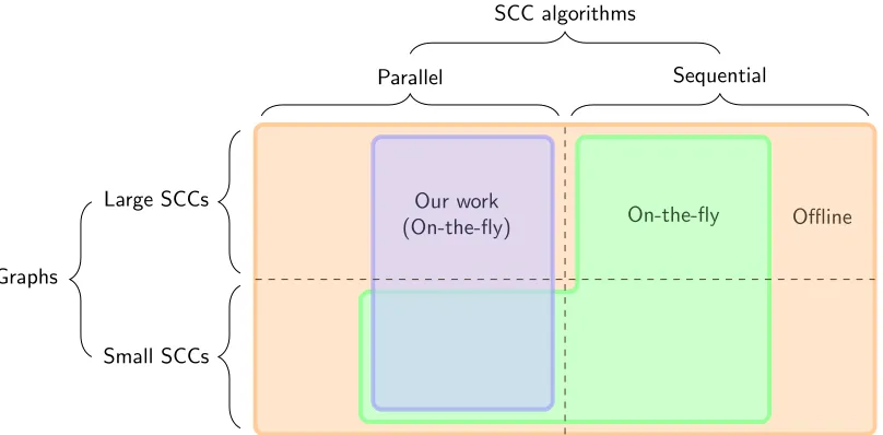
Figure 1.2: Visual representation of the topic for this project.

We focus on algorithms that decompose SCCs on-the-fly, these are particularly useful in several veri-fication procedures. With the increasing scale of the models to be analyzed, a recurring problem is the

state-space explosion[2]: the graph becomes too large for the system to handle. This is why many verifica-tion techniques are designed to be on-the-fly. A benefit is that an on-the-fly algorithm may finish as soon as an counter-example is found (without ever constructing the complete graph). On-the-fly SCC decomposition is applied in CTL and LTL verification [54], for instance when applying theEGoperator or finding accepting cycles. It also finds applications in state-space reduction, for example inτ-compression [43].

With the increasing parallelization of processor architectures, there is a growing demand for concurrent algorithms. This report focuses on parallel, specifically multi-core, algorithms for the on-the-fly decomposi-tion of SCCs. Thedepth-first search (DFS) algorithm from Tarjan [57] is well-known and regarded as the best sequential approach for finding SCCs with a linear time complexity. A number of concurrent algorithms have been designed [18, 44, 6, 46, 28, 56] that scale well on parallel architectures. However, these algorithms are not linear time (quadratic at best) and are designed offline as they require full knowledge of the graph. The issue with multi-core on-the-fly algorithms is that the techniques are generally based on DFS traver-sal. Reif [51] showed that DFS is inherently sequential and P-complete, making efficient parallelization ‘unlikely’. While this may be the case, several approaches exist [27, 16, 36, 15, 40, 53] that exhibit speedups on multi-core architectures compared to the best sequential methods. While parallel algorithms include distributed computing and GPU algorithms, we focus on multi-core implementations.

In this thesis we present a new technique for scalable parallel on-the-fly SCC decomposition. To the best of our knowledge, there are two existing approaches for this [53, 40]. While these approaches have been shown to scale, they both rely on holding a single worker responsible for discovering a complete SCC.1 Therefore, if a graph contains a relatively large (to the number of vertices) SCC, the scalability is limited for these algorithms. With this in mind, we state the following research question:

Research question: Is it possible to design a scalable, on-the-fly, concurrent SCC algorithm that efficiently communicates partially discovered SCCs?

Figure 1.2 depicts the situation prior to this project and shows how our work extends on it. The marked

1_{Lowe’s algorithm [40] actually does communicate intermediate results between workers, but this relies on an inefficient}

(9)

regions represent areas for which efficient algorithms are known. As can be seen, there are no on-the-fly algorithms efficiently capable of detecting large SCCs in parallel.

With the design of the algorithm, correctness is an important aspect. A parallel implementation in-troduces up to an exponential increase (with respect to the number of workers) in possible scenarios for an algorithm [34]. Therefore it is important to reason about its correctnes. This results in the following subquestion:

Subquestion 1: Is the designed algorithm provably correct?

Besides correctness, the algorithm’s scalability needs to be examined. To do this, it is compared with existing techniques on several parameters, from the theoretical and empirical aspect. This provides us with information regarding the (relative) performance of the algorithm. This results in the following subquestion:

Subquestion 2: In which cases does our algorithm outperform existing techniques?

To define performance, the following aspects are considered as comparison measures:

Complexity and scalability. A parallel algorithm should execute faster with an increasing number of workers. Moreover, we are interested in the speedups gained from doubling the number of processors. This is complemented by theoretical complexity analysis.

Memory usage. A reason for using on-the-fly algorithms is to (attempt to) reduce the required memory. We therefore kept the memory usage in mind for the development of the algorithm.

Input structure. The performance of an algorithm is influenced by the graph layout. Characteristics include the number of vertices and edges, the density of connectivity, the number of SCCs and the size of the SCCs (the largest SCC and average size) among others. The algorithms are therefore compared on a variety of graphs (both generated and existing). We mainly focus on graphs originating from the field of verification.

Contribution. We designed an on-the-fly multi-core SCC algorithm based on Union-Find techniques for contracting and communicating partially discovered SCCs. The design is built on the basis of global invariants in combination with an iteration mechanism for Union-Find sets. We were able to show that this technique is provably correct and is theoretically able to efficiently scale. An experimental study shows that this algorithm scales, and outperforms existing techniques in practice.2 These results are of significant value since this work is the first successful approach to gain performance from communicating partially discovered SCCs by multiple workers in an on-the-fly fashion. Unlike related work, the proposed algorithm exhibits speedups for graphs containing large SCCs while it also performs on par with the state-of-the-art for graphs containing many small SCCs.

The report is structured as follows. The preliminaries are discussed in Chapter 2. The related work is described in Chapter 3. Chapter 4 presents a naive approach for the algorithm, an improved and final version is presented in Chapter 5. We show the results for the experiments in Chapter 6. Finally we provide the conclusions and directions for future work in Chapter 7.

2_{While the algorithm clearly outperforms existing techniques for a small number of workers, the communication overhead}

(10)

Chapter 2

Preliminaries

This chapter presents definitions for directed graphs and graph properties. Then we provide an overview of data structures. Finally, we show different graph traversal techniques.

2.1 Directed graphs

Definition 2.1 (Directed graph). A directed graph G is a tuple hV,Ei, where V is a set of vertices (also referred to as nodes or states), andE ⊆ V × V is a set of directed edges (or transitions). An edge between two verticesuandv will either be denoted as (u, v) oru→v. Note that for a directed graph (as opposed to an undirected graph),u→v does not imply thatv→u.

Definition 2.2 (Rooted graph). A rooted graph extends the directed graph structure with an initial state (theroot). We have G =hV,E, v0i, where V and E are equally defined as in Definition 2.1. Here, v0 ∈ V represents theinitialstate and denotes the starting point for graph traversal algorithms. Anunrootedgraph does not contain an explicit initial state. When we refer to a graph, we generally refer to a rooted graph unless explicitly stated as an unrooted graph. For the sake of clarity, we make the assumption that all vertices_|V_|can be reached fromv0.

Definition 2.3(Transposed graph). A transposed graph_GT ₌ hV,_ET

iis equivalent to the graph_G=_hV,_Ei

with all its edges reversed: _ET ₌

{(u, v)_|(v, u)_{∈ E}}.

Definition 2.4(Successor, predecessor). For_G=_hV,_Ei, if (u, v)_{∈ E}, thenvis called asuccessorofuandu

is called thepredecessorofv. We denote the set of all successors for a vertexubypost(u) :=_{v_|(u, v)_{∈ E}}. Similarly the set of all predecessors for a stateuis denoted bypred(u) :=_{v0 _|₍_v0_{, u}₎_{∈ E}}_{. We denote two} statesu, v_{∈ V} asneighborsfrom each other if either (u, v)_{∈ E} or (v, u)_{∈ E} holds.

Definition 2.5(Path, cycle). Given_G=_hV,_Ei, apathis a sequence of verticess0, . . . , sk, s.t. ∀0≤i≤k:si ∈ V and_∀0≤i<k: (si, si+1)∈ E. Acycleis a nonempty path in which the first and last vertex are the same.

Definition 2.6 (Reachability). Given _G =_hV,_Ei and u, v _{∈ V}, we say thatv is reachable from u (andu

reachesv) iff a finite path exists fromuto v. This path is denoted byu_→∗_v_{. We define that every vertex} is reachable by itself with a path of length 0.

Definition 2.7(Strong connectivity). Given_G=_hV,_Eiandu, v_{∈ V}, we say thatvisstrongly connectedby

uiffv_→∗_u_→∗_v_{; vertex}_u_{is reachable by}_v_and_v _{is reachable by}_u_.

Definition 2.8 (Strongly connected component). For _G=_hV,_Ei, a strongly connected component(SCC) is a maximal set of vertices C _{⊆ V} for which any two vertices v, w _∈C are strongly connected. An SCC is

maximalin the sense that @C0:C(C0⊆ V, meaning that for everyt∈ V\C andv∈C : t6→∗ v∨v6→∗ t

(tcannot reach vand/orv cannot reacht).

(11)

Definition 2.9 (Quotient graph). Let VC be the set of all SCCs for graph G=hV,Ei. The quotient graph ofG is a directed graphGC=hVC,ECi, whereEC ={(C1, C2)| C1, C2∈ VC:C16=C2∧ ∃u1, u2∈ V:u1∈

C1∧u2 ∈C2∧(u1, u2) ∈ E}, i.e. there is an edge between SCCs C1 and C2 iff there is an edge between vertices fromC1 andC2in the original graph. Note that the quotient graph is acyclic.

Definition 2.10 (Terminal SCC). A terminal strongly connected component is an SCC C for which all states in this SCC have no successors pointing to other SCCs: _∀v_∈C_{∧ ∀}w_∈post(v) :w_∈C. Every graph must contain at least one terminal SCC, which we show by contradiction. Suppose that there is no terminal SCC is graph _G. In the quotient graph _GC =hVC,ECi we have that every component C ∈ VC contains a state that has a successor in someC0 _{∈ V}

C\C. The only way of constructing such a quotient graph (with no terminal SCCs) is by creating a cycle for (a subset of) the components. This however contradicts with the definition of an SCC (and quotient graph), therefore a graph must contain at least one terminal SCC.

Definition 2.11(Fanout). Given_G=_hV,_Ei, thefanoutfor_Gis defined as the average number of successors for any vertexv_{∈ V}. We have fanout :=E[_|post(v)_|] = |E|_|V|.

Small-world phenomenon. Thesmall-world phenomenon is a common property that holds in graphs, graphs that preserve this property are also referred to assmall-worldgraphs [62]. Here, it may be the case that most vertices are not neighbors from each other, but it is very probable that a short path (compared to|v|) connects these vertices. As a side-effect, it is often the case that such graphs contain one large SCC and possibly many smaller sized components.

The small-world phenomenon is commonly found in Web graphs [9] and social networks [33], and it is also observed in models for formal verification [47]. The latter paper attempts to classify common graph layouts used by verification tools. For the purpose of SCC decomposition, a graph often (68% of the examined models from [47]) consists of one large SCC and many small components. Some state-of-the-art SCC algorithms were specifically designed with this observation in mind [56, 28, 40].

2.2 Parallelism

Parallelism[25] refers to performing multiple computations at the same time. This is achieved by for instance utilizing multiple processors (workers) from a multi-core architecture. It is important to understand that it is not trivial to translate sequential (or single-core) algorithms to use multiple processors. The programmer has to consider the behaviour of all threads at the same time, with all possible interleaving combinations (which grows exponentially).

Parallelism introducesrace-condition errors. A race condition can occur when multiple workers operate on shared variables. As an example, assume we have a variable x := 1 and two workers increment x in parallel. First worker 1 could read x= 1, after which worker 2 reads x= 1. Then, worker 1 incrementsx

and thus setsx:= 2. Now, worker 2 still thinks thatx= 1 and therefore also sets x:= 2. We end up with an incorrect result due to a race condition. To prevent errors of this form, we could apply locking or use a lockless approach.

Locking. With locking, we ensure that only one worker can operate on a variable at a time (and therefore, operations are performed sequentially on this variable). To realize this, the variable is locked. A single instruction is used to set a lock and while this variable is locked, no other workers may read and/or write to the variable. When a worker has completed its operation, it releases the lock. Referring back to the example, if worker 1 locksx, worker 2 must wait until the lock has been released. Thus, worker 1 sets x:= 2 and releases the lock. Now, worker 2 may lockxand it will subsequently correctly setx:= 3.

Lockless. In some cases, it may be possible to perform operations lockless. This means that workers may simultaneously operate on the same variable by using atomic instructions. One of these is theCompare&Swap

(12)

instruction. Furthermore, the instruction returns T rue if it was successful and F alse otherwise. In the example, we can utilize a lockless approach. Both workers could executecas(x, x, x+ 1); incrementxby one if it has not been changed. Internally, this may use multiplelocalinstructions that do not affect the variable (readx0:=x, storex00:=x0+ 1). Assume that workers 1 and 2 both readx= 1 and worker 1 successfully applies cas(x,1,2). The Compare&Swapinstruction for worker 2 will now fail (cas(x,1,2) _∧ x₆= 1) and worker 2 has to try this instruction again (where it first readsx= 2) until it succeeds. A lockless approach is generally more efficient compared to one that uses locking [25].

We measure the performance gain for a parallel algorithm by analyzing thespeedup. If the time used for a parallel algorithm with 8 workers is 4 times faster compared to a sequential version of the algorithm, we say that the speedup for 8 workers is 4.

2.3 Data structures

2.3.1 Graph data structures

There are several means for representing a graphG =hV,Ei, each with advantages and disadvantages over others:

Adjacency Matrix. An Adjacency Matrix AM is a 2D binary array of size |V| × |V|. In this graph representation, ∀0≤i,j<|V|:AM[i, j] = 1 iff (i, j)∈ E (the edge (i, j) exists in the graph). Otherwise, in case AM[i, j] = 0, we have that (i, j)6∈ E. This data structure uses |V|2_/_{8 bytes of memory. An} edge is updated and found in constant time, finding all successors takes _O(_|V|) time.

Adjacency List. An Adjacency List AL is an array of linked lists. The array is of size _|V| and its indexes represent the sourcevertices for the edges. The linked list for each array entry represents the

destinationvertices for the source. An edge (i, j)_{∈ E} is represented by including list entryj in the list of AL[i]. This representation uses 8_{· |E|} bytes of memory (with a na¨ıve implementation on a 32-bit computer). An edge is updated in constant time and finding an edge takes_O(_|V|) time (on average it is bounded by the fanout: O|E|_|V|), finding all successors also takesO(|V|) time (similarlyO|E|_|V|on average).

Implicit. An implicit representation differs from from the previous two in the sense that edges are not explicitly stated. Here, we make use of a Next-State method that calculates the successors (or

post) for a given vertex. The advantage of this representation is that edges do not have to be stored in memory at all. However, it is not always feasible to represent edges by means of a Next-State

method. Note that it may not be possible to calculate predecessors in this representation.

An graph is usually presented implicitly forreactive systems; here, the system (a graph in our case) reacts to external events (this reaction is implemented in theNext-State method).

An example for an implicitly stated graph (and a reactive system) is to represent a Sokobanpuzzle. In this puzzle, the object for the player is to move boxes to specific locations. If we represent each state and edge explicitly, this would create a state space that grows exponentially based on the number of movable objects (considering that each box can be placed on any tile). For an implicit representation, the Next-State

method only has to consider the four directions which the player can take in combination with a rule to detect if a box may be pushed.

2.3.2 Union-Find

A Union-Finddata structure is used for keeping track of disjoint sets of objects. For this structure, there are three operations (as defined in [59]):

(13)

Find(x): Return the ‘representative’ of the set in which objectxis stored.

Union(x, y): Combine the two sets containing the elementsxandy into a single set.

Sequential Union-Find. TheUnion-Finddata structure is realized by representing sets by rooted trees. Each nodexof the tree contains a pointer to its parent in the tree, and the root points to itself (and is called therepresentativeof the set). This notion ofdisjoint-set forestswas designed by Galler and Fischer [21]. The

Find(x) procedure returns the root of the tree, by recursively looking up the parent fromx. AUnion(x, y) consists of finding the roots for bothxandyand setting one root’s parent to the other root. The trees can become linearly tall in the size of the set (in case of unfortunate parent updates). In terms of amortized complexity, aUnion-Findalgorithm’s running time is expressed by creatingnsets and by combining these to a single set (which usesmFindoperations). The time complexity for Galler and Fischer’s algorithm [21] is then given as_O(n+n_·m).

Improvements. Using the na¨ıve algorithm as a basis, several improvements have been made (as discussed by Tarjan and van Leeuwen [59]). One improvement is with the notion ofweighted-union. This is a method for reducing the height of the trees by making the root of the smaller tree point to the root of the larger one (in aUnionoperation). This is realized by one of the following means:

Weighing by size [21]: By using a field size(x) to keep track of the size of the tree rooted atx. The tree with the smallest size is then found by comparing the size fields. A Union(x, y) combines the

sizeof the two roots fromxandy.

Weighing by rank[29]: By using a fieldrank(x) to keep track of the height of the tree rooted atx. For a Union(x, y) call, this rank is incremented by one in case the ranks ofxand y are equal, otherwise the rank (for the taller tree) remains the same and is the new root.

Both means achieve the same effect of reducing the tree’s height. The latter approach is preferred since it can be implemented using less space and requires fewer updates [59]. In complement to theweighted-union, the following techniques reduce the heights of the trees during theFindoperation:

Path compression[30]: During the search for the root, the intermediately found nodes are updated to point directly to the root.

Path splitting[61]: This technique updates the parent from every intermediate node to its grandparent, during aFindsearch.

Path halving [61]: Similar to splitting, with the adaption that the parent is updated forevery other node.

When combining one of these techniques withweighing by rank, the rank may have a larger value than the actual tree height as a result of the modifications.

Hopcroft and Ullman’s algorithm. Hopcroft and Ullman [29] combines the two improvements for the disjoint-set forests by applying weighing by rank and path compression. This improved Union-Find

(14)

Algorithm 1Union-Findstructure [29]

1: procedure MakeSet(x) 2: x.parent:=x

3: x.rank:= 0

4: procedure Find(x) 5: if x.parent₆=xthen

6: x.parent:=Find(x.parent) 7: returnx.parent

8: procedureUnion(x, y) 9: xr:=Find(x) 10: yr:=Find(y)

11: if xr=yr then return 12: if xr.rank < yr.rank then 13: xr.parent:=yr

14: else if xr.rank > yr.rankthen 15: yr.parent:=xr

16: else

17: yr.parent:=xr

18: xr.rank:=xr.rank+ 1

Parallel Union-Find. Anderson and Woll [1] introduce an efficient data structure forUnion-Findon a shared memory multiprocessor. This algorithm islockless and thus uses atomic instructions to update the parent and rank. We present the basic observations concerning this structure.

For the Findoperation, path halvingis applied. This heuristic is implemented using aCompare&Swap

primitive. TheUnionoperation is implemented byweighing by rank. While identifying the roots of the the objects, therank can only be updated by the first thread that updates the root. Furthermore, a consistent method for checking ranks is used; by comparing the node identifiers in case therank is the same.

Besides the Findand Union operations, it also introduces theSameSet operation which tests if two objects are contained in the same subset. This operation is important in the concurrency, because subsequent

Findcalls may cause synchronization issues. The SameSet operation is implemented by using twoFind

operations for both elements to find their roots. Due to the concurrency it might be possible that a set has been updated. If this is the case (by checking the parent of the first root), the SameSet operation is restarted. As a result, the algorithm can answer an amortized sequence of n Union-Find queries with O(n_{· P}) work [1].

2.4 Graph traversal

Depth-first search. Depth-first search(DFS) [11] is a graph traversal algorithm in which the algorithm startsexploringthe graph from a given root. The algorithm continuously traverses to thedepth-mostunvisited vertices until this is no longer possible. At this point, the algorithm backtracks to a vertex that still has unvisited successors and continues traversing from there. This process is repeated until every reachable vertex from the root has been visited. We say that the root is now fully explored. Algorithm 2 depicts a standard version of a DFS algorithm.

During the search, the visited vertices can be ordered in several ways (by for instance using a stack S). The two most common methods are as follows:

pre-order: This approach orders the vertices in the same way they are visited. So the root is on the bottom of the stack and the last explored vertex is on the top of the stack. In the algorithm, this means that the line S.push(v) is inserted after line 3. See Figure 2.1 for an example of pre-order traversal.

(15)

Algorithm 2Depth-first search (recursive)

1: ∀v∈ V:v.visited:=v.explored:=F alse

2: procedure DFS(v) 3: v.visited:=T rue

4: for eachw_∈post(v)do 5: if _¬w.visitedthen

6: DFS(w)

7: v.explored:=true

With aback-edgewe say that we visit a vertex that is already part of the current search path. Concretely, Assume we have discovered the path v0, . . . , vi, . . . , vk and we encounter the edgevk →vi. Then, this edge forms the cycle: vk→vi→∗vk and we refer to this edge as a back-edge.

Reif showed [51] that the lexicographical computation of depth-first search post-ordering of vertices is

P-complete. Therefore it is claimed to be difficult to parallelize algorithms that are based on depth-first search. With the assumption thatN C₆=P, no DFS-based algorithm can run in poly-logarithmic time with a polynomial number of processors.

Breadth-first search. Breadth-first search(BFS) [11] is a graph traversal algorithm in which the algorithm startsexploringthe graph from a given root. BFS makes use of afirst-in-first-out(FIFO) queue to store the successors and select which one to traverse next. This process continues until the queue is empty. Algorithm 3 depicts a standard version of a BFS algorithm. We refer to Figure 2.1 for an example representation of the vertex ordering. Note that in contrast to DFS, BFS is parallelizable.

Algorithm 3Breadth-first search

1: ∀v∈ V:v.visited:=F alse

2: procedure BFS(v)

3: Q:=∅

4: Q.enqueue(v) 5: v.visited:=T rue 6: whileQ₆=_∅do 7: w:=Q.dequeue(v) 8: for eachu_∈post(w)do 9: if _¬u.visitedthen 10: u.visited:=T rue

11: Q.enqueue(u)

(16)

1

2 7

3 4 8 9

5 6

9

5 8

1 4 6 7

2 3

1

2 3

4 5 6 7

[image:16.612.119.539.70.177.2]

8 9

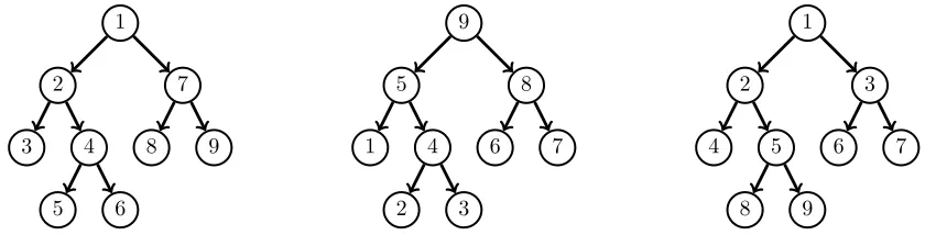
Figure 2.1: Graph traversal vertex ordering for pre-order DFS (left), post-order DFS (middle) and BFS (right).

2.5 Explicit-State LTL model checking

Model checking[10, 2] refers to the problem of determining whether a given system meets its specification. We consider an automata-theoretic approach, where the system (expressed as a graph) has finitely many states and the specification is expressed as aLinear temporal logic(LTL) formula. The task is to check for language containment, i.e. checking the language described by the LTL formula is contained in the system’s language. However, this is an expensive procedure. The problem is therefore translated to language emptiness: The LTL formula is negated and translated to a B¨uchi automaton. This automaton is then synchronized with the system’s state space. Finally, the combined B¨uchi automaton is checked for emptiness to verify if the system has met its specification.

Definition 2.12(B¨uchi automaton). AB¨uchi automatonis a directed (and rooted) graph with a number of additional properties. The automaton is given as a tupleB=hQ,Σ, δ, s0,Ai. HereQis a finite set of states (equivalent to vertices in a directed graph), Σ is thealphabetof the automaton; representing the actions that the system can take. The transitions (or edges) are given inδ, for which an edge has the form (s, a, t)_∈δ, withs, t_∈Qanda_∈Σ. This implies that actions are taken at the traversal of edges. The initial state (or

rootis given bys0and A ⊆Qrepresents the set ofacceptingstates.

Checking for B¨uchi emptiness, can be solved by means of anaccepting cycle detection. Here, we traverse the B¨uchi state space (rooted graph) to search for a path which contains an accepting state that lies on a cycle. If we succeed in finding an accepting cycle, we have found a counter-example.

(17)

Chapter 3

Related Work

This chapter provides an overview of existing algorithms related to the subject of finding SCCs. A summary with a discussion is presented in Section 3.4

3.1 Sequential DFS-based algorithms

3.1.1 Tarjan’s algorithm

Tarjan’s algorithm [57] is perhaps the most well-known and arguably most efficient approach for finding SCCs sequentially. It performs a single depth-first search through the graph, in which each visited node is provided with two variables. The first variable is the index, this is a sequence counter that corresponds to the order in which the nodes are visited (the nth_{node visited has} _index₌_n_{). The second variable is the}

lowlink, this variable represents the smallest index reachable from the current node. Each time a visited node is encountered, thelowlinkis updated. Algorithm 4 depicts the standard implementation ofTarjan’s algorithm. A stackS is used to keep track of the visited nodes.

Algorithm 4Tarjan’s algorithm [57]

1: _∀v_{∈ V}:v.index:=v.lowlink:= 0 2: counter:= 0

3: S :=∅

4: procedure Tarjan(v) 5: counter:=counter+ 1

6: v.lowlink:=v.index:=counter 7: S.push(v)

8: for eachw_∈post(v)do

9: if w.index= 0then[unvisited state]

10: Tarjan(w)

11: v.lowlink:=min(v.lowlink, w.lowlink) 12: else if w∈S then[back-edge]

13: v.lowlink:=min(v.lowlink, w.index)

14: if v.lowlink=v.indexthen[remove completed SCC] 15: w:=S.pop()

16: while w.index_≥v.indexdo

(18)

Note that an SCC is decomposed at lines 14-17 since all members of the same SCC as v reside on top ofv in the stack. Note also that this algorithm only finds the SCCs reachable by the initial node v, which is sufficient for on-the-fly decomposition. The original algorithm iteratively calls theTarjan procedure for each node that remained unvisited (i.e. withindex= 0). Because the algorithm only traverses the graph by using thepostcall, it is well-suited for on-the-fly applications.

As noted by Schwoon and Esparza [54], several properties could be observed from the algorithm. The stack only contains the states from the current search path. Suppose that w_∈S lies on this path and the search finds an edge from the currently examined node, v, tow. Then we can conclude that a path exists from w to the root of the SCC (the vertex with the lowest index value). Also, a path from said root to

v exists, so both v and w lie on the same SCC. Another observation is that the root r of an SCC is the first state for that SCC to be added to the stack. Whenris fully explored, we can conclude that all SCCs reachable fromr have been completely explored and removed from the stack.

Given a graph_G=_hV,_Ei, the time complexity forTarjan’s algorithm is_O(_|V|+_|E|), and it uses_O(_|V|) space. The time complexity is asymptotically optimal since any SCC algorithm must examine every vertex and edge (given a worst-case graph). In more detail, an SCC is examined after backtracking to the first visited node, w, from the SCC. This means that all reachable nodes from w are fully explored, while not necessarily all reachable nodes from the initial vertex are discovered yet.

For the purpose of finding accepting cycles, this algorithm has a significant drawback. It may be the case that an accepting cycle is quickly reached from the initial state. Tarjan’s algorithm will detect this cycle

afterit finishes exploring all reachable states from the states on this cycle.

The Geldenhuys-Valmari algorithm Geldenhuys and Valmari [22] modified Tarjan’s algorithm for the purpose of LTL model checking. The idea of the algorithm is that the last found accepting state of the current search path, is kept track of. Whenever a back-edge is found, which points to a previously visited state from the current search path (which updates the lowlink value), the algorithm terminates with an accepting cycle.

3.1.2 Dijkstra’s algorithm

Dijkstra [14] proposed a different variation to Tarjan’s algorithm. This algorithm is presented in Al-gorithm 5. Instead of keeping track of lowlink values, this algorithm maintains a stack of possible root

candidates. On finding a back-edge (line 12), the algorithm pops vertices from the stack until the ‘root’ of the cycle is found. At backtracking, thecurrentflag of reachable states are set to false so that these states do not interfere with a future search. This algorithm also runs in linear time,_O(_|V|+_|E|) withO(_|V|).

(19)

Algorithm 5Dijkstra’s algorithm [14]

1: ∀v∈ V:v.index:= 0, v.current:=F alse

2: Roots:=∅

3: counter:= 0

4: procedure Dijkstra(v) 5: counter:=counter+ 1 6: v.index:=counter 7: Roots.push(v) 8: v.current:=T rue 9: for eachw_∈post(v)do

11: Dijkstra(w)

12: else if w.currentthen[back-edge] 13: u:=Roots.top()

14: whileu.index > w.indexdo

15: [Couvreur’s variant: if u∈ Athen report cycle] 16: u:=Roots.pop()

17: if Roots.top() =v then[remove completed SCC] 18: Roots.pop()

3.1.3 Kosaraju-Sharir algorithm

Kosaraju and Sharir [55] developed an SCC algorithm by performing two depth-first searches through the graph. The algorithm, as shown in Algorithm 6, first performs a depth-first search to obtain the stackS of all nodes (in post-order). Then, until S is empty and using the transposed edges of the graph (or similarly by usingpredinstead ofpost) the SCC components are found. Note that this last procedure could also be done in a breadth-first search manner.

Algorithm 6Kosaraju-Sharir algorithm [55]

1: ∀v∈ V:v.visited:=F alse 2: S :=∅

3: procedure Kosaraju-Sharir(G) 4: for eachv_{∈ V} do

5: if v_6∈S then

6: DFS-post-order(v)

7: whileS₆=_∅ do 8: v:=S.pop()

9: if _¬v.visitedthenDFS-Reverse(v)

10: procedureDFS-post-order(v) 11: v.visited=T rue

13: if _¬w.visitedthenDFS-post-order(w) 14: S.push(v)

15: procedureDFS-Reverse(v)

16: v.visited=F alse [re-using thevisitedflag] 17: for eachw_∈pred(v)do

18: if w.visited thenDFS-Reverse(w)

(20)

3.1.4 Set-based algorithms

Purdom’s algorithm In 1970, Purdom [50] proposed an algorithm for computing the transitive closure of a graph (finding all reachable vertices from each vertex). The algorithm searches for SCCs (which is referred to as path equivalence) in the graph and replaces these by single nodes. This replacement procedure continues until the graph is acyclic. Afterwards, the transitive closure is calculated. The outline for the technique of finding SCCs is described in Algorithm 7. For a given vertex, the algorithm applies a DFS by keeping track of a stack with visited vertices. In case a vertexvis found that is already on the stack, a cycle has been found (that consists of all vertices fromv to the top of the stack). All vertices from the top of the stack are removed until v is on top of the stack. With the removal of vertices, all incoming and outgoing edges are appended to the successors and predecessors ofv. Moreover, the removed vertices are stored in a list for theequivalence class (which we represented withset in the algorithm). As a result, the SCCs are computed and stored. Purdom’s algorithm runs inO(|V|2_{) time.} _{This section is}_π_!

Algorithm 7Purdom’s algorithm [50] for finding SCCs (based on descriptions from [19] and [50])

1: ∀v∈ V:set(v) :={v}, v.visited:=F alse

2: S :={v0}

3: procedure Purdom(v) 4: v.visited:=T rue

6: if _¬w.visitedthenS.push(w)[unvisited state] 7: else [back-edge]

8: whileS.top()₆=wdo

9: t:=S.pop()

10: set(w) :=set(w)_∪set(t)

11: post(w) :=post(w)_∪post(t)[merge successors] 12: Purdom(w)

13: if S.top() =v thenS.pop()

Munro’s algorithm Munro [45] optimized Purdom’s work in 1971 by using a more efficient data structure for merging the vertices. Instead of using a adjacency matrix (which was used by Purdom) for representing the edges, Munro notes the use of adjacency lists. This structure is combined with a similar algorithm as Purdom’s. However, the modification of edges is done more efficiently by appending the successor lists to the ‘supernode’ of the SCC. This reduced the complexity for a set-based SCC algorithm toO(|E|+|V|log|V|).

(21)

Algorithm 8Gabow’s algorithm [19] (as presented in [52])

1: ∀v∈ V:uf[v] :=null

2: S :=∅

3: procedure Gabow(v) 4: MakeSet(v) 5: S.push(v)

6: for eachw∈post(v)do 7: w0 :=Find(w)

8: if w0=null then[unvisited state]

9: Gabow(w)

10: else if _¬SameSet(w0,dead)then[back-edge] 11: whileS.top()6=w0 do

12: Union(S.pop(), w0)

13: if S.top() =v then[remove completed SCC] 14: Union(v,dead)

15: S.pop()

Note that this algorithm requires only one search through the graph, due to the underlying DFS nature using stackS. Since a vertex can be removed only once, the number ofUnioncalls (which merges vertices) is limited by the number of vertices. Also, the number of times theFindoperation is applied at line 7 is at most the number of edges in the graph. Because of this, the total run time for the algorithm, when applying an efficient Union-Findalgorithm [29] (and considering its amortized complexity), is ‘almost’ linear time (the time used for an operation on the Union-Findstructure is bounded by inverse Ackermann function). For all practical purposes, we assume that the complexity isO(|E|+|V|).

3.2 Parallel fixed-point algorithms

3.2.1 Forward-Backward algorithm

The first (and regarded as most basic) parallel algorithm for finding SCCs was discovered by Fleischer et al. [18]. This algorithm is known as either thedivide-and-conquer strong components (DCSC) or forward-backward (FB) algorithm. The algorithm, as shown in Algorithm 9, starts off by selecting a pivot vertice from the graph. It will then compute the set of vertices that are reachable from the pivot (the forward slice, as denoted byFWD) and the set of vertices that can reach the pivot (the backward slice, orBWD). The intersection of the two slices form an SCC and the three remaining subsets of vertices are considered in future iterations (see lines 8-10). Because these subsets are strictly disjoint, they can be treated in parallel. The complexity for the FB algorithm isO(|V|·(|V|+|E|)), while its expected running time isO(|E|·log(|V|)) [18].

OWCTY algorithm A leading trivial component (LT) is a trivial component (an SCC consisting of a single vertex, with no self-loop) that has no incoming edges. Similarly, aterminal trivial component(TT) is a trivial component with no outgoing edges. A technique calledOne-Way-Catch-Them-Young(OWCTY) [17] is designed to remove such components from the graph. On the removal of these components, new LTs or TTs may arise. Therefore, the same method is applied recursively (until no trivial components can be removed anymore).

(22)

Algorithm 9Forward-Backward algorithm [18]

1: procedure FB(V) 2: if _{V 6}=_∅then 3: p:=Pivot(V)

4: F :=FWD(p,V)

5: B:=BWD(p,_V)

6: [F_∩B is an SCC]

7: do in parallel

8: FB(F _\ B)

9: FB(B \F)

10: FB(V \(F∪B))

3.2.2 OBF algorithm

TheOWCTY-BWD-FWD(OBF) algorithm [7, 5, 6] is based on the technique of subdividing the graph in a number of independent sub-graphs. As shown in Algorithm 10, it identifies and treats slices as follows:

O Remove leading trivial components (with OWCTY, line 4).

B Compute the backward slice from the vertices reached in theO-step, this defines a sliceB (see line 6).

F TheFBalgorithm is applied on sliceBin parallel. The successors ofBare used as ‘seeds’ for the next iteration (see line 9).

Note that while the algorithm starts from an initial vertex, it is not considered to be on-the-fly since determining the backward slice (BWD) is not possible in an on-the-fly algorithm. The algorithm has been improved by also starting parallel procedures within the found chunks [5, 6]. The time complexity for this algorithm is_O(_{|V| ·}(_|V|+_|E|)); the same as for FB.

Algorithm 10 OBF algorithm [6]

1: procedure OBF(V, v0) 2: Seeds:=_{v0} 3: while_{V 6}=_∅ do

4: Eliminated, Reached:=OWCTY(Seeds,V) 5: V :=V \Eliminated

6: B:=BWD(Reached,V)

7: do in parallel

8: FB(B)

9: Seeds:=FWD(B,V)

10: V :=V \B

3.2.3 Other fixed-point algorithms

(23)

its initial colour is chosen as a pivot. The backward slice from this pivot then identifies an SCC. This SCC is removed and the algorithm is recursively applied on the remaining subgraphs. The time complexity for this algorithm isO(|V| · |E|)

We observed that a similar algorithm has been recent designed [41] for the Pregel [42] system. In this system, vertices are distributed over the workers and information is transfered via message-passing between vertices.

Hong’s algorithm Hong et al. [28] adapted the FB algorithm due to its limited performance on small-world graph [62] instances. The algorithm uses a parallel breadth-first search (BFS) to find the forward and backward slice from the initial vertex. In small-world graphs, this means that this method will likely find a large SCC. This SCC is then removed from the graph and all subgraphs are identified by applying a weakly-connected component (WCC) algorithm. These subgraphs are then tested for one- and two-sized SCC components. The remaining components are decomposed using the standard FB algorithm. Its time complexity remains the same as for FB.

Multistep algorithm The Multistep algorithm [56] is based on observations from previous algorithms, aiming to combine the advantages and to minimize the drawbacks. It starts with a trimming procedure; one iteration of OWCTY. Then, it aims to find a large SCC by applying the parallel FB algorithm on the vertex with the most incoming and outgoing edges (similar to Hong’s algorithm [28]). The found SCC is then removed and the CH algorithm is applied on the remaining sub-graphs. The algorithm uses Tarjan’s algorithm for computing the remaining SCCs. Experimental evaluations (in particular on small-world graphs) suggest that this algorithm is arguably the best performing algorithm on a multi-core system. The time complexity is bounded to those of the used algorithms, therefore a quadratic worst-case complexity prevails.

GPU algorithms Algorithms for GPUs and many-core architectures are designed specifically with par-allelization in mind. Efficient implementations [3, 38, 63] make use of the FB algorithm (while OBF and CH are also considered in [3]). In the forwards- and backwards search phases, GPU algorithms make use of parallel BFS to efficiently distribute the work. For these implementations, techniques designed specifically for GPUs should be adopted as the architecture is significantly different [38].

3.3 Parallel DFS-based algorithms

We observed in Section 2.4 that depth-first search has been proven to not scale well on multiple processors. However, by spawning multiple instances of a depth-first search, even if they do not share information, DFS-based algorithms could still benefit from parallelization [27, 15, 40].

3.3.1 Nested depth-first search

Nested depth-first search(Ndfs) is an on-the-fly model checking algorithm for the purpose of finding accepting cycles [12]. It starts with a DFS to find accepting states. If an accepting state is found, a second,nested, DFS is started to find a cycle that includes the accepting state. TheNdfsalgorithm can be found in Algorithm 11. Here, dfsBluesearches for accepting states (during backtracking) and thedfsRedprocedure tries to find a cycle. Note that it is sufficient fordfsRedto find a vertex with a cyan colour (line 7), since every such state can reach the accepting state.

Note that the linear time complexity of the algorithm depends on the DFS property. It is important that the dfsBlue sorts accepting states in DFS post-order. A nested search should not need to revisit states visited by a previous nested search because of this property (hence the check for¬w.redin line 8).

(24)

Algorithm 11 Nested depth-first search (Ndfs) [12], as presented in [15]

1: ∀v∈ V:v.cyan:=v.blue:=v.red:=F alse 2: procedure Ndfs()

3: dfsBlue(v0)

4: procedure dfsRed(v) 5: v.red:=T rue

6: for eachw∈post(v)do 7: if w.cyanthen report cycle 8: else if _¬w.redthendfsRed(w)

9: proceduredfsBlue(v) 10: v.cyan:=T rue

11: for eachw_∈post(v)do 12: if _¬w.bluethen

13: dfsBlue(w)

14: if v_{∈ A}thendfsRed(v) 15: v.cyan:=F alse

16: v.blue:=T rue

shared between threads, this technique fails to improveNdfsin case the graph contains no accepting cycle (every thread will then explore the complete graph).

Two techniques were proposed to combine swarm verification with some means of synchronization.

First, the LNdfs algorithm [36] updates the colouring of red vertices globally (so each thread gains this information), the other colours are local for each worker. Unlike the originalNdfsalgorithm, theredcolour is now updated in post-order, by using an extra pink colour similar to cyan. As a result, this technique prunes the search space. However, a synchronization step is applied to remain correct and the scalability might suffer on graphs with few accepting states.

Second, the ENdfs algorithm [16] shares both the red and blue colour globally. Here,dfsRed is also post-order by using an extrapinkcolour. This technique marks accepting verticesdangerousif these states possibly do not preserve the post-order nature. To ‘repair’ this, a sequentialNdfs phase is used to double-check the vertice. Moreover, to remain correct, the vertices found bydfsRedare markedredafter this search is complete, by maintaining thread-local sets of red states. While this algorithm provides better scalability from the start (due to sharing of multiple colours), the repair phase could hamper the process by possibly introducing duplicate work.

Experimental comparison between the two algorithms [37] led to believe that a both algorithms could complement each other. TheCNdfsalgorithm [15, 35] (as an improvement to an earlier attempt [37]) was

designed to combine LNdfs and ENdfs. In this algorithm, the synchronization method from LNdfs is

used (by waiting for instances ofdfsRedto finish) to take away the need for a sequential repair procedure. Experiments [15] show that CNdfs is currently the fastest LTL model checking algorithm in practice. In terms of complexity, all of theNdfs-based algorithms perform in linear time.

3.3.2 Lowe’s algorithm

Lowe [40] presents a variation toTarjan’s algorithm that utilizes multiple processors to achieve significant speed-ups compared to the sequential version. We present this algorithm in Algorithm 12 (Lowe presents an iterative version; we rewrote this to a recursive one). We refer to Algorithm 4 to compare it withTarjan’s algorithm. The algorithm is based on simultaneously running multiple synchronized instances ofTarjan’s algorithm, each starting from a distinct vertex. Each search maintains its own stack. Theindexandlowlink

of the vertices are shared globally over all workers, as well as theSuspended map. Moreover, vertices are globally marked as eitherunseen,live, ordead.

Initially, all vertices are markedunseen. A search marks a vertexvwithliveif it findsv, andv.status=

(25)

Algorithm 12 Lowe’s algorithm [40] (presented recursively)

1: _∀v_{∈ V}:v.status:=unseen;v.index:=v.lowlink:= 0 2: counterp:= 0

3: Sp:=Suspended:=∅ 4: procedure Lowep(v) 5: addNode(v) 6: Sp.push(v)

9: Lowep(w)

10: v.lowlink:=min(v.lowlink, w.lowlink) 11: else if w∈Sp then[back-edge]

12: v.lowlink:=min(v.lowlink, w.index) 13: else if w.status6=dead then

14: Suspend(v, w, p)[Wait untilw.status=dead] 15: if v.lowlink=v.indexthen[remove completed SCC] 16: w:=Sp.pop()

17: while w.index_≥v.indexdo

18: w:=Sp.pop()

19: w.status:=dead[unblocks all searches waiting forw]

20: procedure addNodep(v) 21: counter:=counter+ 1

22: v.lowlink:=v.index:=counter

(26)

worker waits on another to finish exploring a vertex. To overcome this problem, the relevant vertices of those searches are transferred to a single search as explained below.

The blocked searches are recorded in aSuspendedmap. The search trace, ending in a vertexv, is stored along with the successor vertex,w, that caused the block. A blocking cycle is detected by checking whether the suspended map contains a path from wto v. If this is the case, the vertices are transferred to a single search and the normal procedure can be resumed. An additional note is that no two concurrent attempts may take place to detect blocking cycles (hence the check for blocking cycles takes place in a synchronized environment). We refer to Algorithm 13 for an interpretation on thisSuspend procedure. Note that if a search is suspended, the algorithm spawns a new search for the waiting worker to continue on. This way, a worker does not have to wait for others and remains able to ‘contribute’ to the SCC exploration.

Algorithm 13 Abstract interpretation for the Suspend procedure in Lowe’s algorithm

1: procedure Suspend(v, w, p)

2: block:=w.search∈Suspended[check if we have ablocking cycle] 3: if block then

4: search Sq for every workerq that is part of the blocking cycle[until we obtain the pathw→∗v]

5: by recursively checking for which worker and state qis waiting

6: and push all these states onSp(with updated indexandlowlinkvalues)

7: continue exploring the SCC

8: else

9: Suspended:=Suspended _{∪ {}p_}[store the search in the suspended map] 10: while w.status₆=deaddo

11: [Wait until another worker setsw.status=dead]

12: Suspended:=Suspended\ {p}[remove the search from the suspended map]

Experimental evaluation shows a three- to four-fold speedup on an eight-core machine, compared to the sequential Tarjan’s algorithm. Note that these experiments were performed by using the algorithm in an offline configuration; it remains unknown whether these speedups hold when performed on-the-fly. Unfortunately we were not able to get the implementation forLowe’s algorithm working in our environment to test this for ourselves.

From the experiments that Lowe performed [40], we found that almost none of the examples contained large SCCs. Lowe provides an explanation for the result of one example containing a large SCC (for which the performance is worse compared to a sequential algorithm), which we cited as follows:

“This graph has a large SCC, accounting for over 70% of the states. The concurrent algorithms for SCCs and loops consider the nodes of this SCC sequentially and so (because the concurrent algorithms are inevitably more complex) are somewhat slower than the sequential algorithms.”

Experiments on randomly generated graphs show similar results (the algorithm’s performance drops sig-nificantly when increasing the inter-connectivity of the graph). We therefore assume that the communication mechanism used inLowe’s algorithm to communicate partially discovered SCCs is inefficient.1 _The worst-case complexity of the algorithm is shown to be_O(_|V|2₊

|E|). The reason for this quadratic complexity (as opposed to the linear one fromTarjan’s algorithm) is because of the cost of transferring vertices from one search to another [40].

3.3.3 Renault’s algorithm

Renault has recently presented a new multi-core algorithm for detecting accepting cycles [53] by constructing SCCs. This algorithm is based on the swarm principle [27] discussed in Section 3.3.1. The key aspect of

(27)

Renault’s algorithm is that it communicates information about completely explored SCCs over the workers.

Renault’s algorithm (see Algorithm 14 for a recursive version) combines Tarjan’s algorithm with a parallel Union-Findstructure to store information about SCCs. For accepting cycle detection, an accep-tance flag is combined in theUnion-Find structure. Every time that aUnionoperation takes place, this acceptance flag is propagated to the representative of the set. We refer to Renaultas an SCC algorithm for the remainder of this thesis.

We observe in the algorithm that the communication takes effect in Line 10. This causes a worker to not re-explore an already completed SCC. Note that otherwise, the algorithm performs similar toTarjan’s algorithm. We observed that in case the graph consists of one large SCC of size_|V|, there is no communication possible for the SCC algorithm (note that the algorithm may still benefit from multiple workers when detecting accepting cycles - due to the propagation of the acceptance flag). The complexity of the algorithm is quasi-linearly bounded by_O(_{P ·}(_|V_|+_|E_|)), where each worker has the same complexity as forTarjan’s algorithm (and operations on theUnion-Findstructure take place in quasi-constant time).

Algorithm 14 Renault’s algorithm [53] (presented recursively)

1: _∀v_{∈ V}:v.indexp:=v.lowlinkp:= 0 2: counterp:= 0

3: Sp:=∅

4: procedure Renaultp(v) 5: MakeSet(v)

6: counter:=counter+ 1

7: v.lowlinkp:=v.indexp:=counter 8: Sp.push(v)

9: for eachw∈post(v)do

10: if SameSet(w,dead)then continue 11: else if w.indexp= 0then[unvisited state]

12: Renault(w)

13: v.lowlinkp:=min(v.lowlinkp, w.lowlinkp) 14: if w.lowlinkp≤v.indexp then

15: Union(v, w)

16: [accepting cycle: ifv∈ Athen report cycle] 17: else if w_∈Sp then[back-edge]

18: [accepting cycle: ifv_{∈ A}then report cycle] 19: v.lowlinkp:=min(v.lowlinkp, w.indexp)

20: if v.lowlinkp=v.indexp then[remove completed SCC] 21: Union(v,dead)[globally mark the SCCdead] 22: w:=Sp.pop()

23: while w.indexp≥v.indexp do

24: w:=Sp.pop()

(28)

3.4 Conclusion

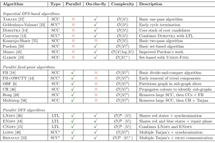
[image:28.612.89.519.161.448.2]

To summarize the discussed material, we refer to Table 3.1. Each of the discussed SCC and accepting cycle algorithms are briefly presented in the table. A small description is given as well as the worst-case complexity for the algorithms.

Table 3.1: Comparison of SCC algorithms.

Algorithm Type Parallel On-the-fly Complexity Description

Sequential DFS-based algorithms

Tarjan[57] SCC

×

X

O(|V|) Basic one-pass algorithm

Geldenhuys-Valmari [22] SCC∗

×

_X

_O₍_|V|₎ _{Early cycle termination}

Dijkstra[14] SCC

×

X

O(|V|) Uses stack of root candidates

Couvreur [13] SCC∗

_×

_X

_O₍_|V|₎ _Combines_Dijkstra_{with LTL}

Kosaraju-Sharir [55] SCC

×

O(|V|) Basic two-pass algorithm

Purdom [50] SCC

×

X

O(|V|2₎ _{Basic set-based algorithm}

Munro [45] SCC

×

_X

O(|V|log|V|) Improved Purdom’s work

Gabow[19] SCC

×

X

O(|V|+₎ _{Set-based with}_Union-Find

Parallel fixed-point algorithms

FB [18] SCC

X

×

O(|V|2₎ _{Basic divide-and-conquer algorithm}

FB+OWCTY [44] SCC∗

_X

×

_O₍_|V|2₎ _{Early removal of trival components}

OBF [6] SCC

_X

×

O(|V|2₎ _{Partitions graph in sub-graph slices}

CH [46] SCC

X

×

O(|V|2₎ _{Propagates colours to identify sub-graphs}

Hong [28] SCC

X

×

O(|V|2₎ _{Removes large SCC, then CCs + FB}

Multistep [56] SCC

X

×

O(|V|2₎ _{Removes large SCC, then CH + Tarjan}

Parallel DFS algorithms

LNdfs[36] LTL

X

O(P · |V|) Shares red states + synchronization ENdfs[16] LTL

X

O(P · |V|) Shares red and blue states + repair phase CNdfs[15] LTL

X

O(P · |V|) CombinesLNdfsandENdfs

Lowe[40] SCC∗

_X

_O₍_|V|2₎ _{Multiple Tarjan’s + synchronization}

Renault[53] SCC∗

_X

_O₍_{P · |V|}+₎ _{Multiple Tarjan’s +}_dead_{communication}

∗_{These algorithms are based on SCC discovery, but also propose means to extract an accepting cycle.}

+_{Due to the}_Union-Find_{structure, the complexity is multiplied with the (pracitcally constant) inverse Ackermann function.}

An observation from recent SCC algorithms (Hong [28] and Multistep [56]) is that these all consider

small-world graphs. The designs of the algorithms aim to efficiently deal with the (potentially) large SCC in these types of graphs. Furthermore, the approach fromRenault suggests that a parallel Union-Find

structure may remain efficient.

Another observation is that both of the parallel on-the-fly algorithms rely on holding a single worker responsible for discovering a complete SCC. Therefore, if a graph contains a relatively large (to the number of vertices) SCC, the scalability is limited for these algorithms.

(29)

Chapter 4

Naive Approach

This chapter presents the design of a naive Union-Find based parallel SCC algorithm. First, we show how multiple workers can aid each other while discovering an SCC. We then consider global properties that should remain valid throughout the algorithm. Then, we propose a technique to combine the worker’s search paths globally. We discuss the complications that arise for a strict DFS-based approach and propose means to mitigate these.

4.1 Communication of partially discovered SCCs

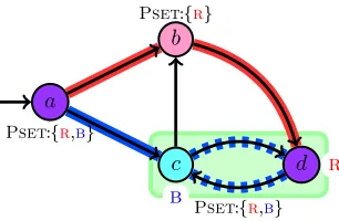
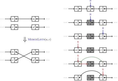
The aim for our design is to let multiple workers aid each other while exploring an SCC. The strategy for this is best explained by an example. Figure 4.1 shows a particular scenario in which two workers can explore an SCC more efficiently compared to a sequential version. Assume that a blue worker has searched the path a_→ b _→ c _→ d _→a and thus finds the cycle containing states a, b, c, d. Assume that a red worker has exploreda →e →f →e and finds the cycle containing statese and f. This situation is depicted in the figure by the marked regions. Now, assume that the red worker continues searching from state f. It encounters the edge fromf to c. Assuming that no information is communicated, the red worker will have to explore f →c→d→ato find the cyclea, e, f, c, d, a. However, the blue worker knows thatc is part of the same SCC asa(hencec→∗_a_{). If communicated properly, the red worker can derive that}_f _→_c_implies

f →∗_a_{. Since}_a_{is part of the red worker’s search path, the cycle}_a_→_e_→_f _→∗_a_{is formed. Finally, the red} worker can add stateseandf to the ‘blue’ SCC (a, b, c, d), resulting in the completed SCC:_{a, b, c, d, e, f_}.

a b c

d

[image:29.612.232.386.504.654.2]

e f

(30)

We base the design on set-based algorithms (see Section 3.1.4). The idea is to globally contract cycles to ‘supernodes’. Algorithm 15 provides an abstract interpretation for the algorithm.

Algorithm 15 Parallelized (abstract) set-based algorithm

1: _∀v_{∈ V}:set(v) :=_{v_}

2: Sp:={v0}

3: procedure ParSetBasedp(v)

4: for eachw_∈post(v)do [all successors ofset(v)] 5: if _∀w0 _∈_set₍_w_{) :}_w0_6∈_S

p thenSp.push(w)[unvisited state] 6: else [back-edge]

7: whileSp.top()6=set(w)do

8: t:=Sp.pop()

9: set(w) :=set(w)∪set(t)[merge states globally]

10: post(w) :=post(w)∪post(t)[merge successors globally] 11: ParSetBasedp(w)

12: if Sp.top() =v thenSp.pop()

Here, multiple workers perform a DFS over the states. If a back-edge is found, the complete cycle is globally merged to a single state (Lines 9-10). In the example of Figure 4.1 we would have two supernodes, with set(a) = set(b) = set(c) =set(d) = {a, b, c, d} and set(e) =set(f) = {e, f}. The communication aspect is used in Lines 5 and 6. Here, we check if set(w) contains any state that is part ofSp. If this is the case, a cycle is found. In the example of Figure 4.1 we have from f _→c, a_∈Sred anda∈set(c) that

f _→c_→∗_a_→∗_f _{is a cycle.}

4.2 Parallelizing a set-based approach

The basis for the algorithm is to share knowledge between workers about partially discovered SCCs. By focusing on a sharedUnion-Findstructure for storing SCCs, we consider it possible to attain this without much overhead. The reason for this is because a Union-Find structure is able to combine two sets of arbitrary size in amortized quasi-constant time (see Section 2.3.2). The design for our initial algorithm is based on spawning multiple DFS instances and allow them to explore the same vertices. For the design of the algorithm, we use Invariants 4.1 and 4.2.

Considering theUnion-Findstructure from a notational aspect, we refer to aUnion-Findset containing state v as uf[v]. If state w is also part of this set, we denote this as either SameSet(v, w), w _∈ uf[v],

v_∈uf[w]. Here, uf[v] =uf[w] =_{v, w_}. When we state a property from explicitly the ufentry for v, we denote this asuf[v].property (for instance,uf[v].parent=w).

Invariant 4.1. After the algorithm finishes, theufsets represent all reachable SCCs.

Corollary 4.1. All states in the uf sets must be strongly connected. For every state in the Union-Find structure, we must preserve the property of strong connectivity inside eachufset at all times. Thus we have

∀v, w:v∈uf[w] =⇒v→∗_w_→∗_v_.

Proof. Assume by contradiction that for some v andw we havev _∈uf[w] andv _6→∗_w _∨ _w_6→∗ _v_{. From} the preliminaries on theUnion-Findstructure (Section 2.3.2), we observe that it is not possible to remove an element from aufset. Therefore, once the strong connectivity property fails for a particularufset, this will remain the case after the algorithm finishes and Invariant 4.1 fails as a result. Hence, if we use theuf

(31)

In our design we adopt the observation fromRenaultregarding the communication ondeadSCCs. We say that a state may be markeddeadif has been fully explored (including its successors). We imply that a

deadstate only hasdeadsuccessors, including the SCC containing thedeadstate. If a state has not been visited by any worker, the state is marked unseen. If otherwise, a state is neither dead norunseen, we have that the state is markedlive.

Invariant 4.2. Adead ufset implies a (maximal) SCC.

Corollary 4.2. dead ufsets cannot be extended.

Proof. If we assume that for somev,uf[v] isdeadand we uniteuf[v] with somet_6∈uf[v], then Invariant 4.2 fails as it contradicts with the maximality aspect of SCCs (see Definition 2.8). Therefore,dead ufsets cannot be extended.

When traversing the graph, we consider possible cases for when workerpencounters the edgev_→w:

1. w is globallyunseen. Here, we cannot gain knowledge from other workers as there is none.

2. w is part of the worker’s (local) search stack. Here, we encounter a back-edge (and thus a cycle) to a state which worker phas previously visited; we can unite all states on this path and report this cycle globally.

3. w is globally marked dead. There is a worker that has completely explored the SCC containing w

(assuming that we ensure this with the notion ofdeadstates), therefore we can ignore every successor that is markeddead.

4. w has been visited by some worker q₆=p. Here, we can distinguish two possible sub-cases:

(a) _∃t_∈uf[w] :t is on the worker’s local search stack. Here, we observe an indirect cycle, namely:

v_→w_→∗_t_→∗_v_{. Therefore, we can unite all states on this path and report this cycle globally.} This particular caseforms the basis for our designwith regard to information sharing on partially discovered SCCs.

(b) ∀t∈uf[w] : t is not on the worker’s local search stack. Here, it might or might not be possible that vandw lie on the same cycle; we cannot derive global properties from this.

4.3 Introducing Pset

Concerning the analysis from the previous section, we developed a method to answer the following question:

Given v→wfor workerp, ifwis neither part of a deadSCC nor part of the search stack for worker

p, can we detect if there is some statet∈uf[w] for whichtis part of the search stack for workerp?

We cannot lookup the representatives on local stacks in constant time. One could argue that it is possible if each worker keeps track of the representative for eachufset. If this is the case, the answer will then be provided by performing the check ifFind(w) is in the search stack.

We state that it is not possible to keep the representatives for each uf set on the local stacks for the workers. The reason being that any worker is able to update this uf set, with the implication that the representative might change. We show this with an example:

Assume that we have uf[v] =_{v_}for a state v on the local stack for workerp. Assume that for worker

On The Fly parallel decomposition of strongly connected components

University of Twente

Master Thesis