Integrated Resources Planning: A Continuous Approach

(1)

Karisa Laras Widyadari

Master Thesis

Integrated Resources Planning:

A Continuous Approach

(2)

(3)

University of Twente

Master Applied Mathematics

Master Thesis

Integrated Resources Planning:

A Continuous Approach

Author:

Karisa LarasWidyadari

Assessment Committee:

Prof. Dr. Marc Uetz,

Dr. Ahmad Al Hanbali,

Dr. Peter J.C. Dickinson,

Dr. Jan-Kees van Ommeren

Integrated Resources Planning: A Continuous Approach

Discrete Mathematics and Mathematical Programming

group of the

University of Twente

(4)

(5)

“You have to be odd to be number one.”

(6)

(7)

UNIVERSITY OF TWENTE

Faculty of Electrical Engineering, Mathematics, and Computer Science

Master of Applied Mathematics

Abstract

Integrated Resources Planning: A Continuous Approach

by Karisa LarasWidyadari

Maintenance logistics is an important area that has been receiving wide attention in scientific literature. Efficient maintenance and logistics can help improve industry’s

and business’ efficiency. In this problem, high availability of resources (spare parts and service engineers) are needed to facilitate corrective maintenance. However, these

resources call for high investments since these resources are mostly expensive. This leads to an interest in efficient cost savings; minimizing the cost while still maintaining to meet the resources availability requirement. Therefore, an optimal resource availability in the

maintenance logistics is needed.

In this master thesis assignment, a service logistics system that involves both spare

parts and highly skilled engineers is considered. Highly skilled engineers are considered expensive assets, thus it is necessary to optimally plan the engineers availability. The

objective is to determine the required capacity of each resource to minimize the total service costs subject to a specified requirement on resources availability. A constrained optimization model has been the developed for the problem by previous work. In this

thesis we formulate the continuous relaxation of the optimization problem. We propose to approach the problem by using logarithmic barrier method. Using this method,

(8)

(9)

Introduction

Maintenance logistics is an important area that has been receiving wide attention in scientific literature [1]. According to [2], ”In today’s global economies, logistics is a key facilitator of trade, and hence an important factor in rising prosperity and welfare”. An

efficient maintenance and logistics system can help to improve industry’s and business’ efficiency.

The importance of maintenance logistics is a result of high investment in assets which require high operational availability. An unplanned downtime of an equipment can be

costly. These unplanned downtimes should be avoided. However, if the unplanned downtimes do occur, the duration should be kept as short as possible to keep a low cost.

This means that unavailable parts or components which cause the system breakdown are immediately replaced by a ready-to-use parts or components. This avoids repairing

a part on site which require too much time.

Therefore, high availability of resources (spare parts and service engineers) are needed

to facilitate corrective maintenance. However, these resources call for high investments since these resources are mostly expensive. This leads to an interest in efficient cost

savings; minimizing the cost while still maintaining to meet the resources availabil-ity requirement. Thus, an optimal resource availabilavailabil-ity in the maintenance logistics is needed.

In this master thesis assignment, a service logistics system that involves both spare

parts and highly skilled engineers is considered. Highly skilled engineers are considered expensive assets, thus it is necessary to optimally plan the engineers’ availability. The

objective is to determine the required capacity of each resource to minimize the total service costs subject to a specified requirement on resources availability.

(14)

Chapter 1. Introduction 2

1.1 Motivation and Research Questions

The motivation for this master thesis assignment has been a paper by Rahimi-Ghahroodi, et al. [3]. In the paper, a constrained optimization model has been developed for the

problem. However, in this master thesis assignment, we approach the service engineers’ queue with a simpler approach, an M/M/E queueing system.

The scope of this assignment is to find an optimization algorithm to improve an existing heuristic method in [3]. Therefore, the general research question for this master thesis

assignment is:

”How to find an optimization algorithm that improves the existing heuristic method for the optimization problem in [3]?”

In this master thesis assignment, we aim to find good solutions using the continuous relaxation formulation of the problem in [3]. Another aim of the master thesis assignment

is to improve the performance of an existing (greedy) heuristic algorithm in [3].

1.2 Approach

In this master thesis assignment, we formulate the continuous relaxation problem of the optimization problem in [3]. We use the extended definition of the Erlang-loss function to non-integral values by Jaganerman ([4], [5]) to replace the Erlang-loss function that

is used in the optimization problem in [3]. Using the Erlang-loss function extension enables applications to nonintegral numbers [5].

In this assignment, we propose to find the solution using the barrier method. With this method, we approach a constrained optimization problem by approximating the

problem using an unconstrained optimization problem. By using the barrier method, we approach the solution from inside the feasible region. The method forms a “barrier”

that prevents the iterated solutions to go outside the feasible region. The unconstrained problem is formulated using a logarithmic-barrier function. In the end, we will implement

(15)

Chapter 1. Introduction 3

1.3 Structure of the Report

This report has the following structure. An overview of relevant literature is given in Chapter2. In Chapter3, we describe the model formulation and state the mathematical

model for the problem. Chapter 4describes the solution approach, in which continuous relaxation problem is introduced and methods are discussed. A complete explanation of

how we implement the methodology described to the problem is explained in Chapter 5 . Finally, in Chapter 6, conclusions and recommendations are given. For an overview of the notations used in this report, the reader is referred to the list of notations at the

(16)

(17)

Chapter 2

Related literature

2.1 Maintenance logistics and Integrated resources

plan-ning

Maintenance logistics is a widely discussed topic in literature [1,3]. One important areas

in maintenance logistics that is extensively studied is the spare part management, partic-ularly the study of spare parts optimization models [1]. A seminal paper by Sherbrooke [6] marked the start of the comprehensive studies, of which he developed a METRIC

(Multi-Echelon Technique for Recoverable Item Control) model. [7] and [8] discuss full overview and techniques to address problems in spare parts inventory control models.

Basten and van Houtum [9] give an update overviews of models in literature on spare parts inventory control, focusing on system-oriented perspective.

Integration of spare parts management and service engineers is rarely considered, how-ever each of these areas have been studied separately in some papers [3]. Several papers

that considered the integration are by Visser and Howes[10] and Hertz et al.[11]. Visser and Howes investigated a model in a service company to determine the optimum number

of maintenance technician to optimize the service company’s profit, while Hertz et al. presented a decision support system that can create simulation models of different field service network, by considering both spare parts and manpower management. Both of

these works use simulation as their performance analysis. In integrating resources, not only spare parts and service engineers, but service tools are often also considered in

repair system. Vliegen discussed the integration between service tools and spare parts planning in her PhD thesis [12]. In her work, she showed that considering the integration of spare parts and service tools lead to more accurate results and saving cost up to 15%,

concluding that integration of different resources planning in maintenance logistics have

(18)

Chapter 2. Related literature 6

high benefits.

This master thesis assignment was motivated by the work in integrated resource planning in maintenance logistics by Rahimi-Ghahroodi et al. [3]. In this paper, both spare parts management and service engineers (manpower planning) are considered. The model is

structured as a queueing model: spare parts queue and service engineers queue. A greedy heuristic procedure is used to optimize the problem. In this master thesis assingment, we

use a simpler queueing model for the service engineers: theM/M/E queueing system. In the model of this master thesis assignment, we assume that the repair calls occur according to Poisson process. This assumption is commonly used in literature. Most of these literature discuss lateral transshipment inventory models. This assumption is

done by Axs¨ater[13], Alfredsson and Verrijdt [14], Kukreja et al. [15], Sherbrooke [16], Kutanoglu [17], Wong, et al. [18], Kranenburg and van Houtum [19]. This assumption is

justified because lifetimes of parts are exponential. This is also justified in the case when lifetimes are non-exponential but the set of systems is so large that the merged stream of failure processes of individual technical systems is close to Poisson [18]. Another

assumption that our model use is that the repair lead-times are exponential. Alfreds-son and Verrijdt [14] used exponential assumption in their work and justified it using

sensitivity analysis.

2.2 Extension of Erlang-loss formula to non-integral

num-bers and its convexity

In this master thesis assignment, we deal with the continuous relaxation of the opti-mization problem of [3]. The aim of this assignment is to find the lower bound on the

solutions. We use the extended definition of Erlang-loss function to non-integral values by Jagerman [4,5].

In [4], Jagerman developed the properties of the Erlang loss function by extending the scope of application of the Erlang loss function to nonintegral numbers and complex

numbers. The extension to the complex plane permits the powerful methods of complex analysis to be applied for obtaining exact, asymptotic, and approximate representations [4]. The convexity proof of the Erlang-loss function (in the domain of the non-negative

integers) had been a known result which was proved by Messerli [20]. Jagers and van Doorn then proved the convexity of the Erlang-loss function extension to non-integral

(19)

Chapter 2. Related literature 7

2.3 The Logarithmic-Barrier method

The Lagrangian relaxation has been used as a method of choice in the related spare part management works by Wong et al. [18], Daskin [22], Diabat [23], Miranda [24], You and

Grossmann [25]. Wong et al. [18] analysed a multi-item, continuous review model of two-location inventory sytems for repairable spare parts. In [18], Wong et al. formulated

a Lagrange relaxation to find the lower bound on the optimal objective function of the original multi-item problem.

In this master thesis assignment, we are interested to find the lower bound of the op-timization problem in [3]. We do this by formulating a continuous relaxation of the

optimization problem. In this master thesis assignment, we propose to approach the solution of the continuous optimization problem by reducing it to unconstrained opti-mzation problem using transformation method. This is done by combining the objective

function and the constraints to form a new unconstrained function whose minimum ap-proximate the solution of the constrained problem [26]. This method is motivated by

practical considerations, since unconstrained optimization problems are easier to handle [26]. One of the procedures for approximating constrained optimization problems by

unconstrained problems is using barrier methods. In this assignment, we use the barrier method to approach the optimization problem. The barrier method is proved to be ”as successful for nonlinear programming as for linear programming” and ”together with

active-set SQP methods, they are currently considered the most powerful algorithms for large-scale nonlinear programming” [27]. In particular, we use the logarithmic-barrier

(20)

(21)

Chapter 3

Mathematical model

In this chapter, the mathematical formulation of the problem, together with the notation, is presented. First, we give a description of the model in section ??. Then, section ??

describes the mathematical formulation of the model. An overview of all parameters,

variables, and functions used in the model can be found in Appendix.

3.1 Model description

The problem in this master assignment is motivated from the problem of integrated resources planning problem in [3]. In this problem, we consider a service maintenance

logistics system that consists of K types of spare parts subject to random failures to store in its local spare parts inventory. Repair calls for spare parts arrive randomly with

rateλ. A repair call of type-krequires one unit of type-kspare part. Each type-krepair call arrives with probability pk with PK_k pk= 1.

The service region has a team of engineers that to do the repair. For each repair call, a service engineer is needed to complete the repair job. In this model, we assume that each

engineer has the same service time regardless the type of repair call that are assigned to them. The service time is the time from a repair job is assigned to a service engineer until the repair job is finished. It is exponentially distributed with rate µ.

When there is no available spare part for repair call type-k, the requested spare parts are satisfied by an emergency channel. When it is the case, both spare parts and service engineers are considered to be satisfied by the emergency channel. This means that the local service engineers are not going to do the repair job.

(22)

Chapter 3. Mathematical model 10

In the case when a spare part is available, a backlogging policy is applied for the service engineers queue. When the spare part is available but there are no service engineer

available to take a repair call request, the system waits until a service engineer becomes available. There is no priority between spare part types, thus the backorders are served

First Come First Served (FCFS). A maximum waiting time is defined for the total waiting time in the service region.

In this problem, we are interested to find the optimal spare parts stock levels and the optimal number of service engineers to minimize the average total cost. In this master

assignment, the problem is restricted under a maximum average waiting time constraint and occupancy rate constraint for the queue model. The waiting times are caused by emergency shipment and service engineers queue. For each spare part, we consider

a holding cost per item per unit. Naturally, the hiring cost of service engineers and emergency cost are also considered in the optimization problem. In section ??, we present the formulation of the model. For a more detailed description of the model, the reader is recommended to see [3].

3.2 Model Formulation

In this section, we give an explanation of the mathematical formulation of the model.

The model in this assignment is motivated by the model in [3]. In section 3.2.1, we present the optimization problem. Following this section, we explain the queueing sys-tems that are involved in the model. In section3.2.2, we briefly discuss the formulation

of the spare parts queue in [3]. In section 3.2.3, we explain the formulation of service engineers’ queue with M/M/E queueing system.

3.2.1 Optimization problem

In this section, we introduce the optimization problem for the integrated resources plan-ning in [3]. Later in Chapter 4, we will describe the continuous relaxation formulation

(23)

min

S,E T C(S, E) =O·E+ K

X

k=1

Hk·Sk+ K

X

k=1

C_kL·ΛL_k(Sk)

subject to W(S, E) = γ

λW

E₊_WS_≤_Wmax

OR(S, E) = γ

Eµ <1 E ≥0, E ∈Z

S= (S1, S2, ..., SK)≥0,S∈ZK

K denotes the number of repair calls type in the problem. The variables are denoted by Sand E. S denotes a vector of (S1, S2, .., SK), whereSk is the stock levels for spare

part type-k, while E denotes the number of service engineers. The components of the optimization problem are explained as follows:

• The objective function T C(S, E)

The objective of this problem is to minimize the total cost needed for the repair

maintenance system. The three parameters in the objective functions areO as the cost of hiring a service engineer per unit time andHkdenotes the holding cost per

item per unit time for spare partk. The last term in the objective function is the emergency shipment costs. CL

k denotes the cost of emergency shipment for repair

callk. We have ΛL

k(Sk) is the emergency shipment rate for repair call typek and

it is a function ofSk. A complete list of notations can be found in Appendix. • The waiting time constraintW(S, E)

The first constraint describes the waiting time constraint of the system. The sys-tem involves two queueing syssys-tems: the spare parts queue and the service engineers

queue. The first constraint describes that the waiting times in the service engi-neers and the waiting time caused by emergency shipment cannot be more than a given maximum waiting timeWmax_.

WS denotes the waiting time that is caused by the emergency shipment. When there are spare parts available in the system, they go to the service engineers queue for the repairing job to be done. The fraction of spare parts that go to

the service engineers queue is described by γ_λ, where γ is the arrival rate in the service engineers queue andλis the total arrival rate of repair calls in the system. Therefore, the waiting time in the service engineers queue is _λγWE_{. A detailed}

explanation of the model in the spare parts queue and the service engineers queue

(24)

• The occupancy rate constraintOR(S, E)

The second constraint describes the occupancy rate requirement of an M/M/c

queue for the service engineers queue, withc as a number of servers (in this case engineers). The occupancy rate gives the server utilization level of the queue system. It describes a stability condition of the service engineer queue. This re-quirement gives a restriction on the stability condition that the arrival of repair

calls can still be handled by the servers (engineers’ service). Violating this con-straint means that the service engineers queue will ’explode’ because the server

cannot handle the rate of incoming repair call arrivals.

In the following sections, we will discuss the mathematical formulation of the queue systems in the model. Section 3.2.2 gives a brief explanation of the spare parts queue

of the integrated resources planning problem in [3]. In section 3.2.3, a description of the service engineers queue will be given. A complete overview of all the parameters,

variables, and functions used in the optimization problem can be found in Appendix.

3.2.2 Spare parts queue

In this section, we give a brief explanation of the spare parts queue formulation of the

integrated resources planning problem (for a detailed description of the model, the reader is recommended to see [3]). In this problem, the spare parts stock replenishment is seen as K “servers” with exponentially distributed replenishment time. In this model, we have exponentially distributed inter-arrival times of repair calls. The queueing system is assumed as anM/M/c/c system. This notation is introduced by Kendall (1953) [28] to denote a queueing model with M denoting exponential interarrival and service time distribution. In this queue system, there are c-server model with Poisson arrival and exponential service time, such that when all the c-channels are busy an arrival leaves the system without waiting for service [29]. This is called a (c-channel)loss system. In this problem, the c servers are the stock level of spare part k, Sk. Thus, we have a

M/M/Sk/Sk queue.

When the stock of spare part k is unavailable, the repair call will be done completely by an emergency service and the repair call is lost. Thus, the probability of emergency service of a repair call is given by the lost probability of M/M/Sk/Sk queue known as

the Erlang-B loss formula. The emergency probability is given by,

P_kL= (ρk

parts)Sk

Sk!

PSk

i=0 (ρk

parts) i

i!

(25)

And the emergency rate of a repair call for spare partk is given by,

ΛLk(Sk) =λkPkL=λk



 

(ρk parts)Sk

Sk!

PSk

i=0 (ρk

parts) i

i!





. (3.2)

withλkdenotes the arrival rate of repair call for spare part typek. When the repair calls

are replenished by the emergency channel, it is done completely by the emergency service

and it must wait until the emergency shipment arrives. This waiting time is important to be considered and is accounted in the accepted waiting times for the repair. For the parts that are supplied by emergency shipment, the average waiting time is equal to

1

νem

k . The average waiting time for emergency channel of all repair calls is the fraction of total repair calls that is satisfied by emergency shipment, times the average waiting

time _νem1

k , given by:

WS =

K

X

i=0

pkP_kL

νem k

(3.3)

withpk denotes the arrival call probability for repair call type-k withPKk pk= 1.

3.2.3 Service engineers queue

We assume exponentially distributed inter-arrival times of repair calls in the service

engineers queue. The service times by E number of service engineers are also assumed to be exponentially distributed. This can be described as an M/M/c queue (Kendall (1951) [28], with M denoting exponential interarrival and service time distribution). The number of servers is again denoted byc, of which in this case is the number of engineers. Thus, in this problem the service engineers queue can be described as anM/M/Equeue. In an M/M/cqueueing system, the occupancy rate is given byρ= _Eµγ . The occupancy rate provides the server utilization level. To have a stable queue, the occupancy rate is supposed to be smaller than one, which can be mathematically expressed as ρ= _Eµγ <

1. This requirement becomes the second contraint in the optimization problem (the importance of this constraint will be thouroughly explained in section 4.3).

(26)

γ =

K

X

k=1

γk= K

X

k=1

λk·(1−PkL) = K

X

k=1

λ−ΛL_k(Sk) (3.4)

We have multiple type of spare parts that arrives in the service engineers queue with

arrival rate λ. In the service engineers queue, we assume that the spare part will be served by exponentially distributed service times that are the same for any type of spare

parts. Therefore, the service rate in the service engineers is the same for all the spare part type, which is given by µ.

When there are no available engineers, the repair calls wait until the first engineer becomes available. In an M/M/E queue, probability of engineers are unavailable can be described by the busy probability for theM/M/E queue [30], which is given by:

PB=

(Eρ)E

E! (1−ρ)PE−1

i=0 (

Eρ)i

i! + (Eρ)E

E!

(3.5)

Simplifying by letting σ=Eρ= γ_µ, (3.5) becomes:

PB =

σE

E! (1−ρ)PE−1

i=0 σ i

i! +

σE

E!

(3.6)

Hence, the average waiting time for the service engineers queue is given by:

WE = P

B

Eµ(1−ρ) =

PB

(27)

Chapter 4

Approach

4.1 Continuous relaxation

In this chapter, we describe how we formulate the continuous relaxation of the problem

in [3]. For this purpose, we need to use the Erlang-B extension to nonintegral numbers by Jagerman [4]. We discuss how we apply this to the optimization problem.

4.1.1 The discrete problem

We reintroduce the discrete optimization problem in [3] introduced section3.2. We call this problem (Z0_):

(Z0) : min

X

k=1

Hk·Sk+ K

X

k=1

C_kL·ΛL_k(Sk)

λW

E₊_WS _≤_Wmax

OR(S, E) = γ

Eµ <1 E≥0, E ∈Z

S= (S1, S2, ..., SK)≥0,S∈ZK

In this thesis assignment, we aim to find a good solution using the continous relaxation

of the problem. Thus we need to formulate the continuous problem (Z0). However, as we have described in section 3.2, optimization problem (Z0) contains the Erlang-B function as the emergency shipment probabilityP_kLin (3.1). In theM/M/c/c queueing

(28)

Chapter 4. Approach 16

system, the blocking probability Pb (Erlang-B function) is usually stated in the form

[4]:

B(x, a) =Pb = ax

x!

Px

j=0 a j

j!

(4.1)

with x denotes the number of servers anda is the occupancy rate or the offered load. As we can see this function contains the factorial and summation which can be difficult

to do when we work with non-integral numbers. In the optimization problem (Z0), we have the blocking probabilityPL

k in (3.1) with (Sk) integers. As we want to formulate a

continuous relaxation problem of problem (Z0), we will have (Sk) to be a positive real

number. Luckily, Jagerman (1974) [4] has introduced the Erlang-B function extension to non-integral numbers

4.1.2 The relaxed problem

In this section we will discuss how we formulate the continuous relaxation problem and

introduce the continuous optimization problem.

Erlang-B formula

In this section, we formulate the continuous relaxation of the problem. For this purpose,

we use the extended definition of the Erlang loss function to non-integral values of x

from Jagerman (1974) [4]:

B(x, a) =

a

Z ∞

0

e−at

(1 +t)xdt

−1

(4.2)

Jagerman (1974) [4] developed an extension of the Erlang-B function to extend the scope

(29)

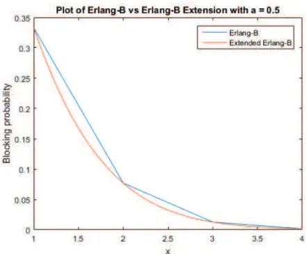
Figure 4.1: Plotting of Erlang-B function (4.1) and the extended Erlang-B function (4.2) for somea= 0.5

Applying the the Erlang-B extension (4.2) to the emergency probability forM/M/Sk/Sk

queue given in (3.1) gives:

P_kL=B(Sk, ρkparts) =

ρkparts

Z ∞

0

e−ρk

partst_{(1 +}_t₎Sk_dt

−1

(4.3)

For the busy probability PB _{of the} _M/M/E _{given in (3.5), we use the relation the}

between the busy probabilityPB _{and the blocking probability of}_M/M/E/E _(Erlang-B

loss function) [29]:

PB = ρB(E−1, σ)

1−ρ+ρB(E−1, σ) (4.4)

With Erlang loss function extension (4.2), this function in turn becomes:

PB= ρ σ

R∞

0 e

−σt

(1 +t)E−1

dt−1

1−ρ+ρ σR∞

0 e

−_σt

(1 +t)E−1

dt−1 (4.5)

(30)

We form a continuous relaxation of the optimization problem. The optimization problem then becomes:

(Z) : min

X

k=1

Hk·Sk+ K

X

k=1

C_kL· λkPkL

λ

PB

µ(E−σ)

+

K

X

i=0

pkPkL

νem k

≤Wmax

OR(S, E) = γ

Eµ <1

with P_kL given in (4.3) and PB given in (4.5). We did not address the constraints

E ≥0 andS= (S1, S2, ..., SK)≥0in this formulation since it is implicitly given by the

remaining constraints.

In the following section, we discuss our approach on solving problem (Z).

4.2 Logarithmic-barrier method

One of the well-known methods for solving constrained continuous optimization problems

is the barrier method (also known as interior-point methods). The barrier method is a procedure of approximating constrained optimization problems using an unconstrained problem, since an unconstrained problem is considered as an ‘easier’ problem to solve

than a constrained problem [27].

Let us consider a constrained optimization problemP:

(P) f(x) s.t. gi(x)≤0, i= 1, ..., m, x∈Rn (4.6)

whose feasible region we denote by:

F :={x∈Rn | gi(x)≤0, i= 1, ..., m}

(31)

minr(θ, x) =f(x) +1

θb(x) (4.7)

withb(x) as the barrier function [31]. 1_θ is the barrier parameter for (4.7). The barrier parameter 1_θ , which is also known as penalty parameter.

A barrier function for problem (P) is any continuous function b(x) that is defined on the interior of the feasible set F such that b(x) → ∞ as limxmaxi{gi(x)} → 0 [32].

The definition of the barrier function indicates that the closer we get to the a constraint boundary, the largerr(θ, x) becomes. Hence, the points that are exactly on the boundary are not defined [32].

The basic idea of the barrier method is to start with a feasible point and a relatively

small value ofθ, which will prevent the algorithm from approaching the boundary. With each iteration, we optimize (4.7) and decrease the parameter value 1_θ monotonically to find a new feasible point. This is done iteratively and at some time, the solution will arrive to a local minimum. We will show in a later subsection that the sequence solution

{xk_} _{converge to a local minimum.}

4.2.1 Logarithmic-barrier function

In this master thesis assignment, we use the logarithmic barrier function that is defined

as:

b(x) =− m

X

i=1

log(−gi(x)) (4.8)

In the logarithmic barrier method, we formulate the inequality constraints into a loga-rithmic barrier term (4.8) in the (unconstrained) objective. Specifically, problem P is

formulated into the unconstrained problem [31]:

B(θ) : minf(x) +1

θ −

m

X

i=1

log(−gi(x))

!

(32)

4.2.2 Convergence

Let the sequence {θk} satisfy θk+1 > θk and θk → ∞ as k → ∞. Let xk denote the

exact solution toP1 forθ=θk, withθkbeing theθof the barrier parameter for function

r(θ, x) at iterationk.

The following lemma gives a set of properties that follows directly from the definition of

xk _{and the definition of the sequence} _{_θ_k}_.

Lemma 4.1. (Barrier Lemma)

1. r(θk, xk)≥r(θk+1, xk+1)

2. b(xk)≤b(xk+1)

3. f(xk₎_≥_f₍_xk+1₎

4. f(x∗

)≤f(xk₎_≤_r₍_θ k, xk)

Proof. See [32].

As previously discussed, the sequence solution {xk_} _{of the logarithmic barrier method}

converge to a local minimum. In fact, the next result gives the convergence of the barrier method.

Theorem 4.2. (Barrier Convergence Theorem)

Suppose f(x), g(x), and b(x) are continuous functions. Letxk_{, k}_{= 1}_{, ...,}_∞_{; be a sequence}

of solutions ofB(θk₎_{. Recall that}_N

δ(x) denote the ball of radiusδ centered at the point

x. Suppose there exists an optimal solution x∗

of P for which N(, x∗

)∩ {x∈R|g(x)<

0} 6=∅ for every >0. Then any limit point x˜ of xk _{solves P.}

Proof. See [32].

4.2.3 Barrier algorithm

In this section we present the barrier algorithm. It is based on solving a sequence of

unconstrained minimization problems, using the last point found as the starting point for the next unconstrained minimization problem. The method was first proposed by Fiacco

and McCormick in the 1960s and was called the sequential unconstrained minimization

(33)

In the following, we present the Barrier algorithm [31] :

Algorithm 4.1 Barrier algorithm

Given: strictly feasible x, θ:θ0 >0, β >1, tolerance >0

Repeat:

1. Compute x∗

by minimizing problemr(θ, x) for θk_.

2. Updatex =x∗

3. Stopping criterion. Terminate if m/θ <

4. Increaseθ. Withθ=β·θ

until stopping criterion is satisfied.

To minimize the problem in Step 1, we use the first-order descent technique, the steepest descent method. We describe the method in detail in the following section.

4.2.4 Descent Techniques

As discussed in the previous sections, to solve the problem (Z), we approximate it by solving an unconstrained optimization problem formulated with barrier method. In this

section, we will discuss the method that we use to solve the unconstrained continuous optimization problem:

minf(x) (4.10)

where f : Rn → R. It is assumed that there exists an optimal point x∗

and f is continuously differentiable. Sincef is differentiable, a necessary and sufficient condition for a pointx∗

to be optimal is:

∇f(x∗

) = 0. (4.11)

see [31]. Thus, solving unconstrained minimization (4.10) is the same as finding a

solution of (4.11), which is a set of n equations in the n variables x1, x2, ..., xn [31].

In this section we will discuss (first-order) descent method that we use to tackle this

problem.

(34)

The descent methods produce a minimizing sequence x(k)_{, k}_{= 1}_{, ...,}_{, where:}

x(k+1) =x(k)+t(k)∆x(k)

and t(k) > 0. In here, ∆x(k) is a vector in Rn. It is called the search direction. The scalar t(k) _>_{0 is called the}_{step length} _[₃₁_{]. The descent methods find}

f(x(k+1))< f(x(k)),

except whenx(k) _{is optimal [}₃₁_{]. In our research, we use the}_{steepest descent method}_.

Steepest descent method

The function f(x) can be approximated by its linear expansion, the first-order Taylor approximation of ˆf(x+v) aroundx:

ˆ

f(x+v)≈fˆ(x+v) =f(x) +∇f(x)Tv.

if v small i.e. if kvk = 1 [33]. Note that if the approximation in the above expression is good, then we want to choose v such that the inner product ∇f(x)T_v _{is as small as}

possible. v is normalized so that kvk = 1. Among all direction v with norm kvk = 1, the direction:

˜

v=− ∇f(x) k∇f(x)k

makes the smallest inner product with gradient∇f(x) [33]. It follows from the following inequalities:

∇f(x)Tv ≥ −k∇f(x)Tkkvk=∇f(x)T

− ∇f(x) k∇f(x)k

(35)

The unnormalized direction ¯v=−∇f(x) is called thedirection of steepest descent at the point x [33]. Let us note that ¯v =−∇f(x) is a descent direction as long as ∇f(x)6= 0, simply observe that ¯vT∇f(x) =−(∇f(x))T∇f(x)<0 as long as∇f(x)6= 0 [33]. The steepest descent algorithm uses the steepest descent direction as its search direction.

The following is the simple steepest descent method algorithm [31,33]:

Algorithm 4.2 Steepest descent algorithm

Given x0, set k= 0

Repeat

• Step 1. vk ₌_−∇_f₍_xk_{). If} _vk_{= 0, then stop.} • Step 2. Choose step lengtht(k) _with _{line search}

• Step 3. Updatex(k+1) ₌_x(k)₊_t(k)_·_v(k)

until stopping criterion is satisfied.

From Step 1 and the fact that vk ₌ _−∇_f₍_xk_{) is a descent direction, we have that}

f(x(k+1)₎_{< f}₍_x(k)_{) [}₃₃_].

4.3 Constraint functions

In this section, we present the analysis on the convexity of the optimization problem. We start by introducing the optimization problem in the case where there is only one

type of spare part in section4.3.1and then in section4.3.2, we investigate the convexity properties of the constraint functions.

4.3.1 Single-item problem

We implement our approach by first considering the case in which there is only one type of spare part. In this way, we can see the problem in the simple case (single stock

type) and analyze the problem before going into multi-item item case. We present the optimization problem in the single-item case:

(Z1) : min

S,E T C(S, E) =O·E+H·S+C

L _λ_·_PL

λW

E₊_WS _≤_Wmax

OR(S, E) = γ

(36)

4.3.2 Convexity properties

In this section, we investigate the convexity properties of the functions in the optimiza-tion problem of the single-item case to give a good idea of the optimizaoptimiza-tion problem’s

properties.

We first approach this by analyzing the constraints and the feasible region of the

op-timization problem to give an idea of the problem before we prove the opop-timization problem’s convexity.

We investigate the properties of the constraint function W(S, E) to give a good idea of the constraint functions. We start by plotting the average waiting time of

emer-gency shipment and the average waiting time of service engineer to see how the function behaves. For this purpose, we use several sample parameters listed as follows:

λ(Total arrival rate) = 0.5

ν (Replenishment rate of sparepart) = 0.4

ρparts (Occupancy rate of spare parts queue) = 1.2

νem _{(rate of emergency shipment) = 10}

µ(Service rate in service engineers queue) = 3

Wmax _{(Maximum accepted average waiting time) = 0.002}

We see in in Figure4.2of the average time for emergency shipmentWS_{, it is decreasing}

as the number of the spare parts increase. This is because when there are spare parts

available, the repair calls would be replenished by the system’s stock parts instead of the emergency channel since the emergency shipment requires a more expensive cost.

This results in the decrease of the waiting time in emergency channel as the spare part stocks increase.

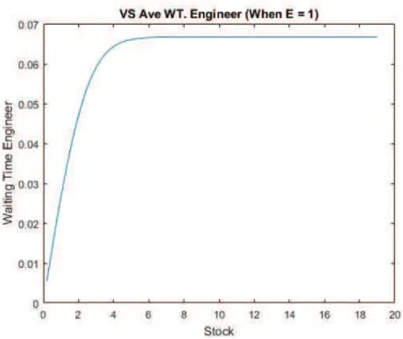
In contrast with the average waiting time for the emergency shipment, the average waiting time for the service engineersWE _{increase as the stock levels for the spare parts}

increase. This happens because when there are more spare parts available in the system, there are more repair calls that go to the service engineers. Figure 4.3 gives the plot

with the number of service engineer equals to 1.

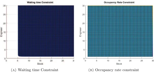
For this case, we also plot the feasible regions of waiting time constraint and occupancy

rate constraint. This figures can be found in figure4.4. Looking at these figure, we can see that the second constraint is redundant, since the feasible region of the problem can

(37)

Figure 4.2: Average waiting time for emergency shipment

(38)

(a) Waiting time Constraint (b)Occupancy rate constraint

Figure 4.4: Feasible region of the case with λ = 0.5, ν = 0.4, νem

= 10, µ = 3, Wmax

= 0.002. The feasible region is indicated by the dark blue color on figure4.4a.

A question arises: what is the importance of the occupancy rate constraint? Since the

feasible region defined by this constraint seems redundant. The following example shed some light on this question. We plot the constraint functions using different parameters. In this case, the arrival rate is much higher than the replenishment rate of spare parts.

The parameters for this plotting are listed as follows:

λ(Total arrival rate) = 4

ν (Replenishment rate of sparepart) = 0.4

ρparts (Occupancy rate of spare parts queue) = 10

νem _{(rate of emergency shipment) = 4}

µ(Service rate in service engineers queue) = 1.5

Wmax _{(Maximum accepted average waiting time) = 0.4}

Figure 4.5 gives regions defined by waiting time constraint and occupancy rate con-straint. In figure 4.5a, we see that there is a fragment (indicated by red color) in the feasible region for the waiting time constraint. Consider the region defined by the

occu-pancy rate constraint given in figure4.5b. This figure suggests that the second constraint in the problem will leave out the fragment in figure4.5a.

To see the reason why this is important, let us consider again the waiting time constraint and the occupancy rate constraint defined by:

W(S, E) = γ

λ PB µ(E−σ) +

1

νem ·P

L_≤_Wmax _(4.12)

OR(S, E) = γ

(39)

(a) Waiting time Constraint (b)Occupancy rate constraint

Figure 4.5: Feasible region with of occupancy rate constraintλ= 4,ν= 0.4,µ= 1.5, andWmax

= 0.4. The yellow region on figure4.5aindicates the feasible region of the problem.

The occupancy rate (4.13) constraint can be rewritten as:

OR(S, E) =E−σ >0 (4.14)

We see that the occupancy rate constraint is no other than the denominator for the waiting time in service engineer queue in the waiting time constraint. The occupancy

rate constraint (4.14) avoids the denominator to become zero of which will make _µ₍P_EB−σ)

becomes infinity, and thus violating the constraint. This constraint also avoids the waiting time becoming negative. Violating constraint (4.14) means that we have the

condition that _Eµγ > 1 of which violates the stability requirement of a M/M/c queue. This stability requirement is needed as violating this requirement means that the queue

will ’explode’ because the server cannot handle the rate of incoming arrivals.

To see this behaviour in detail, we plot the average waiting time of the service engineer’s

queue and compare it as the number of engineers increase. We see in figure4.6, for the case of 1 engineer (blue line) the waiting time ascend sharply before dropping sharply to

a negative number between 4-5 stocks. This also happens to the case with 2 engineers (red line) with the number of stock between 9-10. These sharp ascends happen when

the denominator is approaching zero. The sharp drops indicates that the denominator then starts to become negative, resulting in negative waiting time. Thus, the occupancy rate constraint eliminates the condition when the service engineer’s queue is unstable

(40)

(41)

(42)

(43)

(44)

We will implement the logarithmic barrier formulation (4.15) with the case of 2 spare parts items and 5 spare parts items and see how the solutions achieved with this method

(45)

Chapter 5

Implementation and results

This section deals with the implementation of the logarithmic barrier method to problem (Z). First we present the barrier method algorithm that we use. To analyze whether the algorithm does as what it is expected, we implement it first to a case with single

spare part type. Then we implement the logarithmic barrier method to the case with 2 spare part types and 5 spare part types and see how the solutions achieved with this

method compared to the previous work in [3].

5.1 Algorithm implementation

In this section we discuss how the algorithm is implemented. We explain the imple-mentation into two subsections, the barrier algorithm impleimple-mentation and the steepest

descent method implementation.

5.1.1 Barrier algorithm implementation

In this section, we explain the choice of barrier parameter θ, parameter β that we use in the barrier algorithm.

Choice of parameter β

The choice of parameterβinvolves a trade-off in the number of inner and outer iterations required [31]. Choosing a small β would make each outer iteration θ increases by a small factor, making the previous iterated solution for the Newton steps a very good starting point, which in turn make number of Newton steps needed to compute the next

(46)

Chapter 5. Implementation and results 34

iteration small [31]. We have the opposite situation when β parameter is large. Since after outer iteration θ would increase for a large amount, the current iterated solution would probably not a good approximation for the next iteration [31]. Thus, we can expect more inner Newton steps iteration.

This trade-off in the choice of parameter has been confirmed in both practice and theory [31]. In practice, small values ofβ (near one) results in many outer iterations with just a few steps for each outer iteration. For β large, from around 3 to 100, the two effects nearly cancel, so the total number of Newton steps remains approximately constant [31].

This means that the choice of β is not critical and values around 10 to 20 works well [31]. In our algorithm we choose the β values to be 15.

Choice of parameter θ0

The choice of θ0_{in the algorithm also requires a trade-off in the iteration. Choosing a} large θ0 would make the first outer iteration require too many iterations. When θ0 is small, the algorithm will require extra outer iterations, and possibly too many inner

iterations in the first step [31].

The algorithm4.1is am/t−suboptimal algorithm withmas the number of constraints and a guaranteed accuracy [31]. In this method we take θ0 = m/ and solve the problem using Newton method.

5.1.2 Steepest descent implementation

We use the first-order gradient method, the steepest descent method, to minimize

prob-lem ( ¯Z) in step 1. A discussion of the steepest descent method has been given in section 4.2.4. In this section we describe the search direction and the step length that we use in the steepest descent method in our algorithm.

Search direction

The direction of locally steepest descent is given by:

sk =−(Ak)−1

∇M(xk)

(47)

For our algorithm, the search direction that we use is defined as:

sk=−∇Z¯((S, E)k) (5.1)

by choosingAk ₌_I_{, the} _n_×_n _{matrix. Since,} _I−1

=I, we obtain5.1.

Step length

For computing the descent step length δk_{, we use the nonoptimal step alternative. In}

the nonoptimal step, we find δk _{which satisfies:}

M(xk+δksk)≤M(xk) (5.2)

By using the nonoptimal step, it increases the computational efficiency since more com-putation would be needed to find δk _{that satisfy} _M₍_xk₊_δk_sk_{) = min}

δM(xk+δksk)

[26]. However, in our algorithm, we use the optimal step with the last barrier parameter. For optimization along the line (xk₊_δk_sk_{), we use the sequential halving search [}₂₆_].

This procedure is similar to a procedure for finding the real roots of an algebraic or transcendental function [26]. In this method, the interval to be searched is halved and the portion wherein the objective functions are smallest is retained [26].

5.2 Single-item case

In this section, we explain the implementation to the case of single spare part type. The

purpose is to have a good idea on how the algorithm works. We present two different case for the implementation. The parameters that we use for this implementation is

described as follows:

Parameters Case1 Case2

Arrival Rate of Repair calls (λ) 4 0.5 Rate of spare part replenishment (ν) 0.4 0.4 Rate of Engineer’s service time (µ) 3 12 Rate of Emergency shipment (νem₎ ₁₀ ₁₀

Cost of Engineer (O) 700 900 Holding Cost of Spare part (H) 500 500 Cost of Emergency Shipment (CL₎ ₅₀₀₀ ₅₀₀₀

Maximum Waiting time (Wmax₎ _0.05 _0.03

(48)

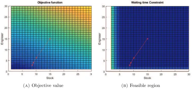
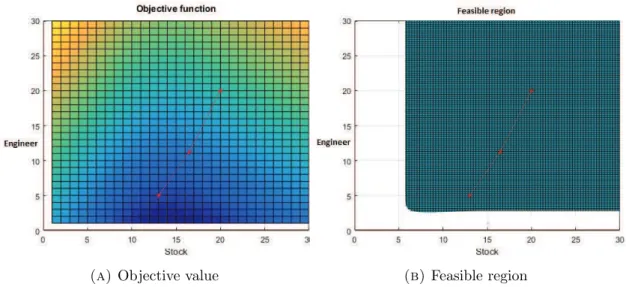
(a) Objective value (b)Feasible region

Figure 5.1: Objective value and feasible region for case 2. The darker the color in figure5.2a, the smaller the objective value.

We present region plotting of the objective value and the feasible region for both cases. In the pictures, we see there are different colors on the region. These colors represents

the value difference of the plotted function. The darker the color the smaller the value is.

We see from the two sets of figures, for both case 1 (Figure5.1) and case 2 (Figure5.2), the iterated solutions go towards the minimum since they go towards the darkest region

of the objective value. For case 1, we see in figure 5.1b, there are lighter colored area. These indicates that the value of the waiting time is near the maximum waiting time,

even though these are still feasible. We can also see from Figure 5.1b, how the barrier “effect” comes into play as the iterated solutions (indicated by red dots) refused to go near lighter colored area. For case 2, the iterated solutions also go towards the minimum

and the solution is feasible.

From both of the cases that we present, the iterated solutions from the algorithm is working as it is expected. This means that iterated solutions go towards the minimum and barrier prevents the iterated solutions to go outside the feasible region. However,

we should note that from these two example that the iterated solutions may not produce the lowest total cost as the barrier may prevent in doing so.

(49)

(a) Objective value (b)Feasible region

Figure 5.2: Objective value and feasible region for case 2. The darker the color in figure5.2a, the smaller the objective value.

5.3 Multi-item case

In this section we implement the barrier algorithm to the multi-item case and present the results. In particular, we implement the algorithm to 2 spare parts case and 5 spare

parts case. As the aim of the assignment is to provide an improvement of the solutions in the previous work in [3], we implement the solutions from the barrier algorithm as the

initial solutions for the heuristic algorithm in [3]. To make both problems comparable, the heuristics algorithm is adjusted so that the formulation assumes Poisson process as in our model. We will call the solutions as the Barrier-Heuristic solutions. Then, we

will compare the barrier-heuristic solutions with the original heuristic solutions and see whether there is an improvement in the solutions achieved.

In general, we compare 3 different solutions in this section: the barrier algorithm solu-tions, original heuristic solusolu-tions, and the barrier-heuristic solutions.

In this section, we present the results of the implementation. We implement this to 150

different cases for to achieve solutions for 3 methods: the barrier algorithm, original heuristic algorithm, and the barrier-heuristic algorithm.

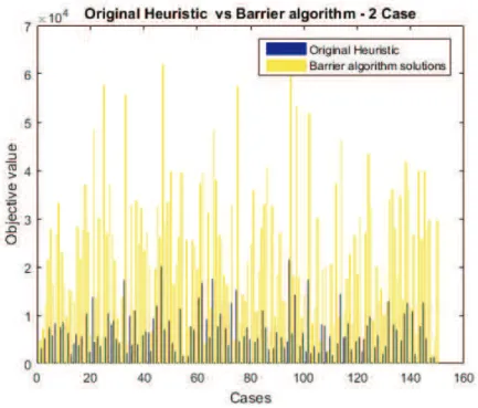
Barrier algorithm solutions vs Original heuristics solutions

First, we implement the barrier algorithm to solve the continuous optimization problem

( ¯Z) to the case of 2 items and 5 items of spare parts. In the 2 spare parts case, the barrier algorithm did not perform as well as the simple case. The algorithm produce

(50)

The average difference of the total cost is 23105,22. It seems that the algorithm does not work as well in more variables as it is in the simple case. For the 5 spare parts case, the

difference of the total cost is 41594,655. The high difference is caused by some variables that are far too large compared to the heuristics solutions. A possible explanation is

that this happens because of the nonconvexity of the problem or that the barrier comes into play. Based on these results, in both 2-item and 5-item case, the barrier algorithm never produce better solutions compared to the original heuristics.

To solve one case, the barrier algorithm takes on average 40.778 sec for 2-item case and

105.167 sec for 5-item case. The results from the barrier algorithm can be found in table 5.2. Figure 5.3 and 5.4 represent the comparation over the achieved result for 2 spare parts case and 5 spare parts case, respectively.

Barrier algorithm 2-item case 5-item case

Average difference of total cost to original heuristic 23105.22 41594.655

Average computational time to solve 1 case 40.778 sec 105.167 sec

Table 5.2: Average difference of Barrier algorithm solutions compared to original heuristic solutions

(51)

Figure 5.4: Comparison on original heuristic algorithm solutions and barrier algo-rithm solutions in 5 items case

Barrier-heuristics solutions vs Original heuristics solutions

To see whether the achieved solutions on the barrier algorithm make an improvement on the original heuristic algorithm, we apply the barrier algorithm solutions to be the

starting points for the heuristic algorithm. Since we solved the solutions of a continuous relaxation problem, we round the solutions to the nearest integer. This is done so that it

can be applied to the heuristics algorithm that solves the discrete optimization problem. We applied this for 150 different data for both 2 and 5 items.

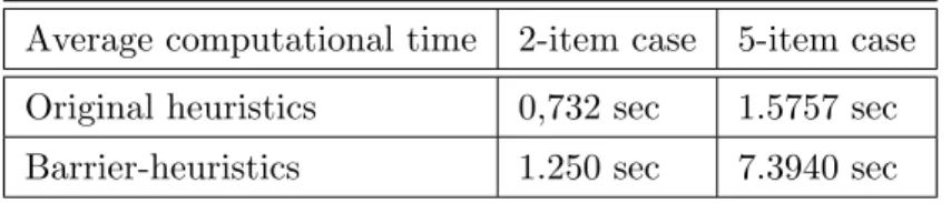
The computational time for the barrier-heuristics seems to perform less well than the heuristic algorithm, although the difference is relatively small. We did the test by

running the algorithm to solve 150 cases. For the 2-item case, the original heuristic algorithm takes on average 0.732 seconds, while the barrier-heuristic takes 1.250 seconds.

(52)

Average computational time 2-item case 5-item case

Original heuristics 0,732 sec 1.5757 sec

Barrier-heuristics 1.250 sec 7.3940 sec

Table 5.3: Average computational time of Barrier-heuristics vs Original heuristics in seconds

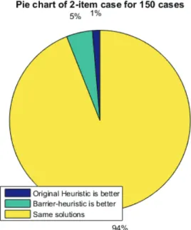
Although the barrier-heuristics takes more computational time, some solutions produce

better solutions than the original heuristics method. In 7 out of 150 cases, the barrier-heuristics produce better solutions than the original heuristic algorithm, with a difference

of 727,339. However, there are 2 cases where the original heuristics produce better solutions than the barrier-heuristic solutions. For the rest of the cases, both methods give the same solutions. This might be the case that the solutions are already optimal.

Table 5.4 presents the results of the comparation for 2-item case. A pie chart of the results produce by the two methods is given in figure 5.5.

2-items Barrier-heuristics Original heuristics

Number of better solutions 7 2

Percentage of better solutions 4.67% 1.33% Average difference of better solutions 727,339 905,877

(53)

Figure 5.5: Pie chart on original heuristics solutions and barrier-heuristic solutions in 2-item case over 150 cases

Similar results are also found when we compare both methods on the 5-item case. In 10

out of 150 cases, the barrier-heuristics give better solutions than the original heuristic method. Although, we also found that in 6 cases, the original heuristics give better

solutions than the barrier-heuristics solutions. For the rest of the problem, the solutions from both method is the same. Again, this might be the case that the solutions are already optimal. The results are given in table5.5. A pie chart on the solutions achieved

by the two methods can be seen in figure5.6.

5-items Barrier-heuristics Original heuristics

Number of better solutions 10 6

Percentage of better solutions 6.67% 4% Average difference of better solutions 1236,839 2987,719

(54)

Figure 5.6: Pie chart on original heuristics solutions and barrier-heuristic solutions in 5-item case over 150 cases

We have presented the results of using the barrier algorithm to approach good solutions

(55)

Chapter 6

Conclusions and further research

This section will describe the conclusions that can be drawn from the results of this

research and the recommendations for improvements and further research.

6.1 Conclusions

In the following, we consider the research question and answer this question by drawing the conclusions from this research. The research question is:

“How to find an optimization algorithm that improves the existing heuristic method for the optimization problem in [3]?”

In this research, we propose to do a continuous relaxation of the original discrete problem

in [3] and find a good solution on the problem. We use the barrier method to approach the solutions of continuous relaxation problem. The barrier method approach the

solu-tions of the problem by approximating the constrained problem using an unconstrained problem, because an unconstrained problem is easier to solve. It approaches the solution from inside the feasible region, which guarantees the achieved solutions to be feasible.

However, from the results of the barrier algorithm in Chapter 5, it is shown that the achieved solutions do not approach a good solution in the case of 2-item and 5-item

spare parts. The solutions are feasible, however, they are not better compared to the heuristic solutions. It might be the case that the barrier “effect” comes into play or the fact that the optimization problem is generally a non-convex problem. In conclusion,

the barrier algorithm still needs to be improved to be able to achieve better solutions.

We apply the solutions of the barrier algorithm to the original heuristic algorithm

and compare the results to the original heuristic solutions. We call the solutions as the barrier-heuristic solutions. Time-wise, the original heuristic is still faster than the

(56)

barrier-heuristics algorithm. For the solution comparation, although the original heuris-tics still produce better solutions than the barrier-heuristic solutions in some cases, there

are also cases where the barrier-heuristic solutions have better results. In the cases where the barrier-heuristic give better solutions, it might be the case that the solutions of the

barrier algorithm are better starting points than the one from the original heuristics. For the rest of the cases, the barrier-heuristics solutions have the same solutions as the original heuristics solutions. This might be the case that the solutions are already

optimal.

Based on these results, we conclude that although the solutions from the barrier

al-gorithm still do not give better solutions than the original heuristic solutions, these solutions do give some improvements when they are used as the starting points for the original heuristics algorithm. However, we should also note that there are cases where

the original heuristics give better solutions. We also note that the barrier algorithm still needs to be improved to give better solutions and computational time. Consequently,

this may also improve on the computational time for the barrier-heuristics method. In the following section, some recommendations for further research is presented.

6.2 Further Research

In this section, recommendations for further research based on the research is discussed.

6.2.1 Second-order Descent method: Newton’s method

For the current research, the barrier algorithm is implemented using the steepest descent method. Due to time limitation for conducting the research, we did not extend our discussion to the second-order descent method. For further research, it would be good to

apply the second-order descent method, the Newton’s method, for the barrier algorithm. The Newton’s method uses the second-order derivatives of the objective function. Thus,

in some cases, it can give faster convergence than the gradient descent because it takes less iterations to the local minimum. Using the Newton’s method may improve the

computational time of the barrier algorithm.

6.2.2 Merit function

As we have an optimization problem that is generally a non-convex problem, it may

(57)

determine whether a step is productive and should be accepted. This may improve the achieved solutions of the barrier algorithm.

6.2.3 Starting points feasibility

The barrier algorithm requires feasible point as its starting point. There might be cases where these points are not known. For further research, we suggest to take this into account by extending the starting point to infeasible starting points. This can be done

(58)

(59)

Appendices

(60)

(61)

Notations

Parameters

• K : Number of spare parts.

• O : The cost of hiring a service engineer per unit time

• Hk : The holding cost per item per unit time for spare partk • CL

k : The cost of emergency shipment for repair callk • λ: Total repair call arrivals.

• pk : Probability that the repair call needs type-k spare part. • λk =pk·λ: Arrival rate of repair call type-k.

• νk : The replenishment rate of spare part typek.

• ν_kem : The replenishment rate of for emergency shipment for spare part type-k.

• ρparts_k = λk

νk : The offered load in spare parts queue.

• µ: The service rate of service engineer.

Variables

• Sk : Non-negative variable that indicates the stock level of spare part type-k. • E : Non-negative variable that indicates the number of service engineer.

(62)

Functions

• The emergency rate of a repair call for spare part k(ΛL k):

ΛL_k(Sk) =λkPkL=λk



 

(ρk parts)Sk

Sk!

PSk

i=0 (ρk

parts) i i!   .

• Arrival rate in service engineer’s queueγ:

γ =

K

X

k=1

γk= K

X

k=1

λk·(1−PkL) = K

X

k=1

λ−ΛL_k(Sk)

• The offered load in service engineers queue:

σ= γ

µ

• The probability of emergency shipment:

P_kL= (ρk

parts)Sk

Sk!

PSk

i=0 (ρk

parts) i

i!

• Average waiting time of emergency shipment (WS_):

WS=

K

X

i=0

pkP_kL

νem k

• Average waiting time in service engineer’s queue (WE_):

WE = P

B

Eµ(1−ρ) =

PB

(63)

• Total Cost (the objective function):

T C(S, E) =O·E+

K

X

k=1

Hk·Sk+ K

X

k=1

C_kL·ΛL_k(Sk)

• Waiting time constraint:

W(S, E) = γ

λW

E₊_WS _≤_Wmax

• Occupancy rate constraint:

OR(S, E) = γ

(64)

(65)

Acknowledgements

In this section of my master’s thesis I would like to thank and express my gratitude

to those who helped me to complete this work, finalize my studies and stood by me throughout my studies here in The Netherlands.

First and foremost, I would like to my parents and brother. Without their prayers and endless support, I would not be able to overcome the challenges that I have faced. I

hope we meet again soon.

I would also like to thank my grandfather, Waloejo DS. He has been the biggest supporter

on my academic journey so far and have always believed in me, even when I don’t.

Agung, for being one of my closest friend throughout my study in The Netherlands.

Luna, I’m glad we met and have become best friends ever since we met on both the Bandids band and the orchestra.

Lulu, for always listening to my rants and stories. I hope I have been doing the same.

Thank you to Mas Rully, Mas Riswan, Citra, Bayu, (and again, Luna). Thank you for

letting me be a member of The Bandids band. It was an honor to be in the band and represent Enschede with you guys. Our journey to get the title of “The best Indonesian student band in The Netherlands” have been one of the most memorable memories in

my study. And I do know for sure that this is one of the reason that keep me sane throughout my study here in Twente.

Tanja and Marieke, for letting me to be in the same group with them in the first semester in 2014/2015 academic year. Now, they are one of my closest friends in the

applied mathematics program and I’m grateful for that.

Eefje Schut, for her companion throughout the process of doing my master thesis.

Peter, for being my daily supervisor. Thank you for your advice and patience with me.

Sajjad, for his advice and patience on explaining his work to me.

Thank you to the assessment committee members, Marc Uetz, Ahmad Al Hanbali, and Jan-Kees van Ommeren for their time to assess my master thesis.

(66)

Integrated Resources Planning: A Continuous Approach

Karisa Laras Widyadari

Master Thesis

Integrated Resources Planning:

A Continuous Approach

University of Twente

Master Applied Mathematics

Integrated Resources Planning:

A Continuous Approach

UNIVERSITY OF TWENTE

Master of Applied Mathematics

Abstract

Contents

This work is dedicated to my family. Thank you for being the best

supporters throughout the years.

Chapter 1

Introduction

1.1

Motivation and Research Questions

1.2

Approach

1.3

Structure of the Report

Chapter 2

Related literature

2.1

Maintenance logistics and Integrated resources

plan-ning

2.2

Extension of Erlang-loss formula to non-integral

num-bers and its convexity

2.3

The Logarithmic-Barrier method

Chapter 3

Mathematical model

3.1

Model description

3.2

Model Formulation

Chapter 4

Approach

4.1

Continuous relaxation

4.2

Logarithmic-barrier method

4.3

Constraint functions

Chapter 5

Implementation and results

5.1

Algorithm implementation

5.2

Single-item case

5.3

Multi-item case

Chapter 6

Conclusions and further research

6.1

Conclusions

6.2

Further Research

Appendices

Notations

Acknowledgements