Floater Allocation in Paced Mixed Model Assembly Lines: Design and implementation of a method for operational scheduling of cross trained workers in Mixed Model Assembly Lines

(1)

i

Floater Allocation in Paced

Mixed-Model Assembly

Lines

Design and implementation of a method for

operational scheduling of cross-trained workers in

Mixed-Model Assembly Lines

Master Thesis

Tjarco van Overbeek

May 2015- December 2015

Supervision University of Twente

1st supervisor: Dr. Ir. J.M.J. Schutten

2st supervisor: Dr. Ir. M.R.K. Mes

Supervision Ergo-Design

1st supervisor: Ir. P. Hentschke

Faculty & Educational program

Faculty of Behavioral, Management and Social Sciences

Master Industrial Engineering and Management

Track Production and Logistics Management

(2)

i

Summary

This thesis considers a paced Mixed Model Assembly Line (MMAL): an assembly line that handles multiple configurations/models of a product (cars in this thesis) that are transported with a constant speed. The time each station has to finish its activities is referred to as the takt of the line. Workers move alongside the assembly line while working on the product.

In these MMALs, stations see varying workloads. In the search of a high level of utilization, MMALs are often designed such that the average processing time at each station is approximately equal to the takt (Scholl, Kiel, & Scholl, 2010). This results in situations in which station cannot finish its activities on time. Workers can move out of the regular station bounds to keep working on the car. However, the distance that a worker can move out of a station (called overlap) is limited, due to availability of parts and/or power tools. When the car reaches the end of the overlap, the worker is forced to move back towards the beginning of his station to start working on the next car. The amount of seconds that a station falls short in completing its activities is referred to as overtime in this thesis, and every occurrence of overtime counts as one defect.

The client (referred to as Company A), has indicated that line stops and lowering the feeding/transportation pace of the assembly line are not desired options to resolve these situations. This is where floaters step in. Floaters are cross-trained workers who provide temporary support to ‘busy’ stations. In the current way of working, floaters are employed reactively, responding to requests for help from stations. This results in sub-optimal usage of floaters, missing opportunities to resolve overtime. Therefore, the goal of this thesis is: To develop a tool for the operational scheduling of floaters in the assembly line of Company A, with the goal of minimizing overtime and defects in the final assembly.

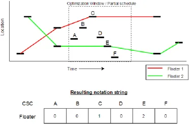
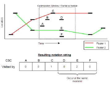
We created a model that uses Car/Station Combinations (CSCs) as basis. Each CSC ‘occurs’ in a fixed timeframe: from the moment the car enters the station until it leaves the station. Help can only be provided by floaters within this timeframe.

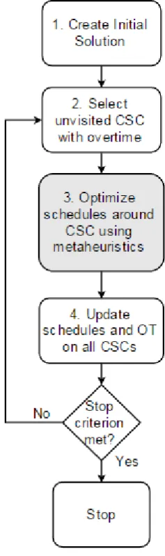
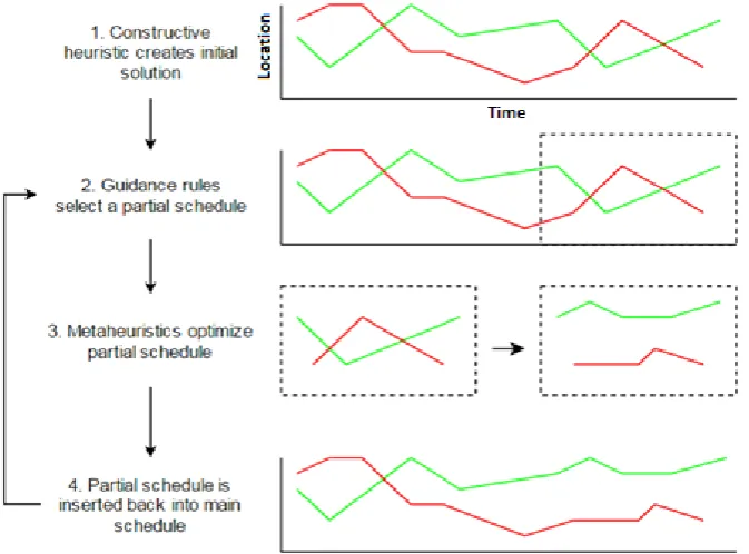
The assembly line is divided into working areas that each have an assigned number of available floaters. We create schedules for each working area separately. Our proposed solution method first creates an initial solution using a Parallel First Come First Serve heuristic, resulting in a schedule for all available floaters. This initial solution is then further optimized, by iteratively taking out small parts of the floater schedule in which problems occur, called partial schedules, and optimizing them using Simulated Annealing. The quality of a floater schedule is determined by calculating the objective function with the form(𝑤1 ∗ ∑𝑂𝑣𝑒𝑟𝑡𝑖𝑚𝑒 + 𝑤2 ∗ ∑𝐷𝑒𝑓𝑒𝑐𝑡𝑠).

We implemented the solution method and carried out a numerical analysis to determine the optimal settings for the parameters of the methods.

(3)

ii

Foreword

Before you lies my master thesis, which marks the end of my master’s programme Industrial Engineering and Management (‘Technische Bedrijfskunde’ in Dutch). In this thesis, I developed a method to schedule cross-trained workers, called floaters, in a paced assembly line. Floaters provide support to stations along the assembly line that are too busy. The challenge is to schedule floaters such that they resolve as much problems as possible. In the scheduling process travel times have to be taken into account, as the assembly line

considered in this thesis covers a total area of 300 meters long and 200 meters wide.

I have enjoyed working on this assignment for several reasons. The assignment was challenging, based on a real case, and gave me the opportunity to walk through a complete process; from formulating a model and solution methods to evaluating and optimizing the performance of those methods.

This thesis would not have been possible without the help of several persons. First, I thank the persons at Ergo-Design, the providers of the assignment. Paul Hentschke acted as my external supervisor, and was always open to talk about the assignment. The basis of this assignment is a model, and one can sometimes forget what a model represents: reality. Paul helped a great deal in making sure the final solution method would be useful in practice. I also thank the owners of Ergo-Design, Jaap Westerink and Douwe Bonnema, for giving me the opportunity and the resources to make this assignment possible. Their positivity and flexibility made working at Ergo-Design a very pleasant experience.

Next, I thank my supervisors at the University of Twente, Marco Schutten and Martijn Mes. I enjoyed the mix of criticism and positive feedback during our meetings. Considering the number of graduate students they were supervising at the same time, I was surprised by the level of thoroughness by which they reviewed my work. The feedback and insight provided by Marco and Martijn helped to improve the quality of this thesis.

Finally, I thank my family, girlfriend, friends and roommates for their support. Especially those who had to put up with me rambling on about my assignment. If I mistakenly thought that you were still interested after the first minute, I apologize.

(4)

iii

iv

5.7 Total solution configuration ... 69

5.8 Benchmark ... 71

5.9 Total solution performance ... 71

5.10 Influence of objective function on overtime and defects ... 72

6. Discussion, Conclusions and Recommendations ... 73

6.1. Discussion ... 73

6.2 Conclusions ... 75

6.3 Recommendations ... 76

6.4 Suggestions for further research ... 78

References ... 79

Appendices ... 81

Appendix A: Abbreviations and Vocabulary ... 81

Appendix B: Screenshot of floater scheduling frame in Plant Simulation ... 82

Appendix C. Results of Hill Climbing algorithm on Working Area 4 and 7 ... 83

Appendix D. Results of Simulated Annealing on Working Area 4 ... 84

Appendix E. Results of Simulated Annealing on Working Area 7 ... 85

Appendix F. Linear Regression result for SA parameter settings on Area 4 and 7 ... 86

Appendix G. Optimization of Parameters for Genetic Algorithm ... 87

Appendix H. Results of Genetic Algorithm on Working Area 4 ... 90

Appendix I. Results of Genetic Algorithm on Working Area 7 ... 91

Appendix J. Iterations of improving GA ... 92

Appendix K. Experiment for Guidance Rules ... 92

(6)

1

1. Introduction

This thesis was written as part of a graduation internship at Ergo-Design B.V. in Enschede. This company is currently developing a simulation based day-to-day planning system for the final assembly at a car

manufacturer that we shall refer to as Company A in the remainder of this thesis. Any (information or) images used in this thesis are chosen in a way that conceals the company’s identity. The final assembly at Company A is done on an assembly line that can handle multiple models of cars with different configurations, called a mixed-model assembly line (MMAL). The goal of this graduation assignment is to contribute to the planning system, by developing a tool for scheduling cross-trained workers (called floaters) to assist regular workers on the assembly line. The model is being developed for a single plant, but the possible deployment of the package at other facilities has been taken into consideration by Ergo-Design.

In this chapter, an introduction is given to Ergo-Design and (mixed-model) assembly lines in Section 1.1 and 1.2 respectively. Then the challenges that arise on these assembly lines are introduced in Section 1.3. Possible methods of dealing with these challenges are discussed in Section 1.4. In Section 1.5 the problem is described and the scope is defined, resulting in the research plan in Section 1.6.

1.1 Ergo-Design B.V.

Ergo-Design is a consultancy company that specializes in Industrial Engineering. It was founded in 1991 and has 14 employees. Its operating areas can be grouped by factory design, lean production, and logistics and planning as shown in Figure 1. Activities of Ergo-Design consist of developing master plans for production facilities and logistic networks, and designing plant and production line layouts. Other activities include optimizing efficiency, logistics, quality, and ergonomics, performing simulation studies and developing smart scheduling applications such as takt clocks and digital scoreboards. References (among many others) include Scania, Volvo, Volkswagen, NAM, Akzo-Nobel, Tata, Thales, and Bosch.

1.2 Company A

Company A is a car manufacturer that uses an assembly line for the final assembly of their cars. An assembly line is “a flow-oriented production system where the productive units performing the operations, referred to as stations, are aligned in a serial manner” (Boysen, Fliedner, & Scholl, 2007). The assembly line at Company A can assembly different models and configurations of cars on the same line, with batch sizes as small as one and negligible set-up times in between. This is called a Mixed-Model Assembly Line (MMAL). MMALs provide several challenges (discussed in Section 1.3), and to cope with these challenges Company A has decided to develop a day-to-day planning system together with Ergo-Design. This planning system will simulate production runs based on input data such as which cars to produce on a certain day. The model will then provide

processing times and other data that can be used to make an efficient production plan for that day. In this thesis we develop a tool that will be added to the total planning system. The tool will be used to schedule cross-trained workers to assist regular workers on the assembly line in an optimal way.

MMALs are employed in many production industries where flexibility is required. In the light of the problem at hand, we mainly refer to the application in the automotive industry in this thesis.

(7)

2 1.3 Challenges in MMALs

In Mixed Model Assembly Lines, products require different processing times on each station depending on their specification. In order to achieve an acceptable level of utilization, the line is designed such that the average processing time (at each station) is approximately equal to the takt of the line (Scholl, Kiel, & Scholl, 2010). As a result, labor intensive (‘hard’) products will have processing times longer than the takt at certain stations, whereas those of ‘easy’ models will be shorter. An assembly line is called balanced if the average processing times on all stations is approximately the same.

On the one hand, production companies aim for a high utilization to keep costs low. On the other hand, a high utilization means that imbalances on the line (differences in processing times) will lead to capacity overload situations, where a station cannot finish the product within one takt. The extra time the station needs to finish its activities is called overtime. Each occurrence of overtime is called a defect. Sometimes overtime can be resolved by regular workers by walking along the line outside the bounds of their working area. The distance that workers can walk outside their working station is called ‘overlap’. This distance is limited, due to availability of power tools and limited working space. If the overtime cannot be resolved, then the work that remains unfinished has to be repaired either along the line (at a touch-up station) or after the product leaves the assembly line. These repair activities are costly as they require extra personnel and processing time. The main objective is to acquire a high utilization without deteriorating the assembly line performance in terms of quality and costs resulting from rework.

1.4 General solutions

In order to face the challenges mentioned in Section 1.3, imbalances on the line have to be prevented or compensated. There are several ways to do this.

The first option is called line balancing (Ghosh & Gagnon, 1989). Each station has a set of tasks assigned to it, such as installing a sunroof or an automatic transmission. Line balancing focusses on allocating these tasks to stations in a way that minimizes capacity overload situations by dividing workload as equally as possible (see Section 3.2). This process is generally done as part of medium or long term planning as it can involve relocating power tools and personnel or redesigning working areas. Inputs for line balancing are predicted product demand, the precedence relations of tasks and their processing times. As a result of changing demand, variations in working speed, defects in parts or malfunctioning power tools, it is hard to perfectly balance a mixed model assembly line. Line balancing cannot be carried out every day, and peaks in workload will remain that have to be resolved using short-term oriented methods.

The second option is product sequencing (Ghosh & Gagnon, 1989), where the sequence of products to be sent down the line is chosen (see Section 3.2). Given the allocation of tasks determined by line balancing, the processing times of cars on each station can be determined. By cleverly constructing a sequence, the resulting workload can be leveled for each individual station to a certain degree. For example, cars with a large workload at a certain station can be followed by one with a small workload at that station, to give the station time to ‘catch up’. This is a simplified view on product sequencing, as the effects of changing the sequence become less clear as the number of stations increases.

(8)

3 1.5 Problem and Scope

Revisiting the previous section, we now describe the scope of this research and the reasoning behind it. The planning system developed by Ergo-Design is aimed at day-to-day planning. Therefore line balancing has fallen out of scope as this is a medium/long term activity that should not be carried out daily. The next step is product sequencing, which has already been carried out and implemented in the planning system (Op Den Kelder, 2015). After line balancing and product sequencing, overload situations still occur on the assembly line. Line stops and altering line/feeding speed are options that come at the cost of productivity, which is undesirable and has been indicated by Company A as such. The last remaining option to solve overload situations is the employment of floaters, which is the focus of this research (see Figure 2).

The scope of this research is thus limited to the scheduling/allocation of floaters in the final assembly of Company A. It is assumed that required materials are at the right place at the right time. We consider the allocation of tasks to each station and their duration as given, in compliance with the planning system that has been developed so far. In this thesis, the sequence of cars is considered as given.

1.6 Research plan

We have discussed the general context and problem(s), and we have defined the scope of the research to be the scheduling of floaters in the final assembly. Currently floaters are already being used by Company A but in a reactive way without planning beforehand (see Section 2.3). Company A feels that they would benefit from an operational planning for floaters, and therefore the goal of this research is:

To develop a tool for the operational scheduling of floaters in the assembly line of Company A, with the goal of minimizing overtime and defects in the final assembly.

In order to successfully do this, we need to answer the following research question:

What is the best way to allocate floaters in a Mixed Model Assembly Line, in order to minimize overtime and defects?

(9)

4

We divide this question it into sub questions and answer them one by one. First, we must learn more about the assembly line (configuration, properties, etc.) and how floaters are scheduled in the current situation. Also, more knowledge of the planning system that has been developed so far is needed, in order to come up with an appropriate solution. In Chapter 2 we tackle the first research question:

1. What does the final assembly at Company A look like? 1.1 What is the configuration of the assembly line? 1.2 What are its properties?

1.3 How are floaters scheduled in the current situation?

1.4 What are the contents of the planning system and how does it work?

This step is taken before the literature review, as we do not need specialized knowledge to describe the current situation, and more insight in the production process allows us to review literature in a more focused manner. We review literature in Chapter 3 to see what earlier work has been done in relation to the scheduling of floaters, and what methods have been or can be used to solve this problem.

2. What methods can be used to schedule floaters in MMALs according to the literature? 2.1 What is a Mixed-Model Assembly Line?

2.2 What is the role of floaters in MMALs?

2.3 How has the scheduling of floaters been dealt with in the literature?

2.4 Which problems related to floater scheduling are known in the literature, and what methods can be used to solve them?

2.5 What other methods can be used to solve the optimization problem in this thesis?

With the knowledge we have gathered from previous research questions as input, we can now construct a solution method in Chapter 4, answering the following research question:

3. What method is best suitable for minimizing overtime in the assembly line of Company A? 3.1 What are the functional requirements to the solution design?

3.2 What are the technical aspects of the problem?

3.3 How should the current situation be translated into a model? 3.4 What methods should be used to solve this model?

3.5 How can the solutions be validated, e.g., how do we assure feasibility?

Now we have determined the method(s) that will be used for solving the floater scheduling problem, we implement them in the current planning system. Next, their parameters must be set, and the performance of the proposed solution method must be tested. Therefore we answer the following research questions in Chapter 5:

4. What are the optimal values for the different parameters of our methods, and how does the total solution method perform?

4.1 What plan should we use to set the different parameters?

4.2 What are the best settings for the parameters used by our solution method? 4.3 What can be used as benchmark for the performance?

4.4 What is the performance of the total proposed solution/method?

4.5 How sensitive is the provided solution method to changes in key variables?

(10)

5

2. Current Situation

In this chapter, a detailed description of the final assembly process at Company A is given. This answers the first research question, provides insight in the assembly process, and enables us to focus on relevant literature in Chapter 3.

2.1 Assembly line configuration

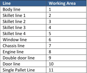
The production process under consideration is the final assembly at Company A. Cars are assembled on an assembly line, where workers use tools to perform manual jobs, such as installing the engine or doors. It is a mixed-model assembly line, meaning that different versions of cars can be produced on the same line, with virtually no set-up times in between. The assembly line consists of a total of 15 production lines that have a total of 222 workstations. It is a labor intensive process, and in total there are 343 regular workers active in the final assembly. A detailed subdivision is given in Table 1.

Line # of workstations # of fixed

workers

Assembly examples

Body zone line 6 12 Tank and locks

Skillet line 1 21 28 Hood, suspension

Skillet line 2 21 40 Harness

Skillet line 3 23 30 Alarm, side windows, and bumper

Skillet line 4 20 38 Gear shift and handbrake

Window line 1 4 6 Windows

Chassis line 71 94 Fuel line, exhaust, radiator, oil reservoir

Engine line 18 25 Engine

Double Door Line 10 12 Doors

Door Line 4 8

Subassembly line 1 24 50 Door speakers, door, mirrors Subassembly line

2,3,4 & 5

Are part of the final assembly, but work without takt times and therefore fall outside the scope

Total # 222 343

Table 1. Elements of assembly line at Company A

A ‘car’ that enters the assembly line is a frame that somewhat resembles a complete car. An example of such a car frame is given in Figure 3.

(11)

6

Before a car can be put on the road, a lot of components need to be installed. For nearly every component there are a number of options available. For example, a car can be bought with an optional air conditioning or sunroof. In this production process, the configuration of each car is stored in a so called ‘80 column row’. Each column represents an option, and the character in that column describes which option has been chosen for this specific car. An example of the 80 column row is given in Figure 4.

Figure 4. Example '80-column-row' for options

The amount of possible options per station differs from a minimum of one option to a maximum of 55 options. The current average number of options per station is 16.4. It becomes clear that a large number of different configurations are possible. The workload at a station for a given car depends on the options that are chosen. For example, a station installing the sunroof will have no workload if this option has not been chosen.

In this thesis we make the assumption that all parts are available for each car to be assembled. In reality, this assumption may not hold as suppliers might fail to deliver on time or certain parts have defects. Cars for which certain parts are missing will be removed from the list of cars that are available for production. Cars are selected from this list to enter the final assembly, and therefore cars will only enter the assembly line if all parts are available for assembly.

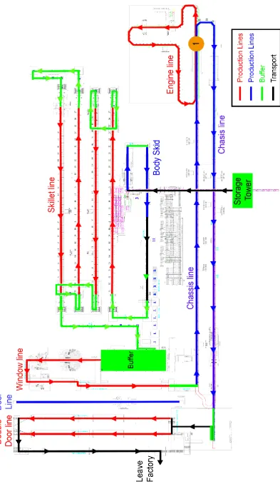
In Figure 5 a layout of the total final assembly is shown. Cars are stored in the storage tower before entering the final assembly. The cars are retrieved from the storage tower using an AS/AR system, and then flow through the assembly line following the arrows as shown in Figure 5. The sequence in which the cars are selected from the buffer tower is also the sequence in which the cars will flow through the assembly line, and stays the same for the entire process. The cars move through the body, skillet and window lines before

(12)

[image:12.595.101.495.69.755.2]

(13)

8

Figure 6. Assembly line flowchart

2.2 Assembly line properties

In Section 2.1 the general characteristics and layout of the assembly line were discussed. In this section, the detailed properties of the line are discussed.

Takt

In this assembly line a takt time is used of 52.8 seconds. Stations must finish their activities within this

timeframe. Stations have a length between 3.5 and 7.5 meters, and the line speed at these stations is such that the car will leave the station after 52.8 seconds. Stations have different lengths because of requirements for room for tools and personnel.

Storage tower and buffers

The storage tower that precedes the final assembly has a maximum capacity of 730 cars. Based on a takt time of 52.8 seconds, the line is able to assemble 68.2 cars per hour. The maximum number of cars that can be produced in an 8 hours shift is 545, and there are 2 shifts per day.

Buffers have been placed between the different lines indicated with the color green in Figure 5. These buffers can be seen as empty stations, and cars will flow through them in the same rate (one per 52.8 seconds) as through the stations. These buffers can be seen as decoupling points in the assembly line, meaning that any overtime from the stations before the buffer have no effect on the stations after the buffer. This would only be possible if a worker would walk along the line through the whole buffer to complete his activities, which is realistically not possible because the ‘walk-along’ distance (or overlap) is limited to a distance that is much smaller than the buffers.

Lines, Stations and Workplaces

(14)

9

Figure 7. Lines, Stations and Workplaces

Frequency

Sometimes the best option is to let a single worker perform a job, instead of multiple workers. A reason for this can be that the working area is limited (a hard to reach location in or on the car) or the task at hand is

indivisible. If this is the case, ‘frequency’ is used as a solution. This means that instead of having 3 workers (for example on workplaces L1 thru L3 in Figure 7) working on the car simultaneously, one worker moves with the car along the workplaces. More than one worker is put in a station, and each worker processes a car

alternately.Worker number one processes car 1, and walks along with the car through the all the workplaces in the station. Worker number two works on car 2, and so forth. The station length might also be increased to give the worker enough time to finish the activities. If there are X workers doing their work as described above, the ‘frequency’ of the station is 1/X.

Double door line

As mentioned earlier, the double door line consists of two parallel lines. This is done because the processing time on most of its stations is approximately twice the takt. One line processes the even cars and the other processes the uneven cars. This gives the stations on each line double the time to complete their activities.

2.3 Workers and floaters

Each station in the assembly line has a minimum of one regular worker assigned to it. This worker has the required competences to work at this station (each station requires different competences). Workers are part of a team, which is assigned to a part of the assembly line.

Next to regular workers, floaters are used in the assembly line. These floaters are cross-trained workers that have the required competences for a part of the assembly line, and can work at any station in that zone. Most often these floaters are team leaders, but dedicated floaters are also used. Floaters can provide help at stations in case of a capacity overload, in order to reduce overtime. Currently there is no offline operational planning for the floaters. If an overload situation occurs in the line, a floater is requested at the station. If a floater is available at that point in time, it will move to the station to provide help. Floaters are assigned on a first come first serve basis.

2.4 Planning system

(15)

10

2.4.1 Goal of the planning system

The planning system has been developed to cope with the challenges that were discussed in Chapter 1. As mentioned earlier, line balancing is time consuming and cannot be performed on a daily basis, or for every change in demand. That is why an operational planning is needed to resolve remaining overload situations. Given a fixed allocation of tasks to stations, Company A performs production planning which determines the sequence of cars and the allocation of floaters. To support this process the simulation model was developed, with the goal of:

 Quantifying the effects of changing the sequence of cars that will be sent down the line, and constructing methods to construct efficient sequences (sequencing).

 Quantifying the effects of different allocation rules for floaters, and developing methods to schedule floaters in the assembly line in an optimal way (floater allocation).

We now discuss the contents and the functionality of the model. 2.4.2 Contents and Functionality

The current planning system is constructed in Tecnomatrix Plant Simulation. This software was developed by Siemens PLM Software and allows users to gain insight into their production processes by modelling them and simulating production runs. The model contains the final assembly as a whole and all lines and buffers that have been discussed in this chapter have been modelled. Workers are assigned to the stations and perform their activities as cars move over the line.

Production data is loaded into the model, which contains the cars that are in the storage tower. After it has been determined which cars will be produced and an initial sequence has been made (based on simple rules), the simulation is conducted. During the simulation relevant data are recorded that can be used for analysis. The starting/ending time of each car on each station is registered together with the processing time, used capacity, capacity overflow, and idle time per worker. It is possible to zoom in on parts of the assembly line for more details. Workers in the model change color according to the workload they are facing. Workers can change color ranging from blue (little workload) to dark red (high workload). This gives a visual indication of stations that have trouble keeping up with the takt.

After the simulation is completed, the processing times of the cars on each station can be used to optimize the sequence of cars that will be sent down the line (see ‘Sequencing’ section below). Based on this sequence floater allocation can be performed. The process of gathering information and performing optimization using the model is shown in Figure 8.

(16)

11

Sequencing

The first goal of the simulation model is related to sequencing. In the old situation, sequencing for the assembly line was done purely based on mixing rules. Some examples of mixing rules are: only one in three cars can have a sunroof, only one in four cars of model x, and a maximum of two cars with air-conditioning in every four consecutive cars. Company A used 40 of such mixing rules. These rules have been developed to reduce overload situations in the assembly line, and are developed using a certain demand of cars. When this demand changes, the mixing rules become inefficient, resulting in (more) overload situations. Also mixing rules can result in a residual of difficult cars that remain unscheduled. Sequencing based on mixing rules had already been adapted into the simulation model in an automated way, in order to increase the speed of creating sequences and testing them by simulating the production run.

In the current planning system, a product sequencing module has already been developed (Op Den Kelder, 2015). Using the processing times that are produced by the simulation model, the sequence of cars was improved in order to reduce peaks in workload. To this extent, Op Den Kelder (2015) applied several heuristics such as Simulated Annealing to swap cars in the sequence and evaluate if this would decrease overload situations. In this way, a sequence of cars is constructed that minimizes overtime.

In this thesis, the sequence of cars to be sent down the line is considered as given. The optimized sequence that results from the methods of Op Den Kelder (2015) will be used as input in determining an optimal floater schedule/allocation.

Floater allocation

The second goal of the simulation model is to allocate floaters in an optimal way. As discussed earlier, there is no operational planning for the floaters yet, as they are assigned to stations while the assembly line is running by team managers. The simulation model provides possibilities to change this. Because the cars that have to be produced on a certain day are known in advance, overload situations in the line can be predicted given a sequence of cars and the allocation of tasks to the station (which is static).

With this information, it becomes possible to make a planning that makes the best use of floaters, e.g., each floater resolves as much overtime as possible. In this planning, travel distances and time can be taken into account to determine what overload situation can be reached from a certain station at a certain moment. If methods are developed for allocating these floaters in an optimal way, the company can then investigate what the effect is of increasing the number of available floaters for a production zone.

2.5 Conclusion

In this chapter the current situation in the final assembly of Company A has been described which provided insight into the configuration and properties of the final assembly. The current practices related to the allocation of floaters has been discussed.

The current method of floater allocation is done reactively without planning beforehand. If an overload situation occurs in the assembly line, the line manager assigns a floater (if one is available) to help resolve this issue. The allocation of floaters is done on a first come first serve basis, which may result in sub-optimal use of the floaters. More overtime can possibly be resolved if overload situations can be predicted and floaters can be scheduled accordingly.

(17)

12

3. Literature review

In this chapter, the existing literature that is relevant for this research is reviewed. In Section 3.1 we give an introduction to MMALs. In Section 3.2 and Section 3.3 literature is reviewed to determine the role of floaters in MMALs and what methods have been developed to schedule them. In Section 3.4 we discuss problems related to the problem of Floater Allocation in Mixed Model Assembly Lines (FAMMAL). In Section 3.5 we discuss and solution methods for the Vehicle Routing Problem (VRP). Finally, we discuss metaheuristics that are used to provide solutions to complex problems.

3.1 (Mixed Model) Assembly lines

The modern version of the assembly line was first utilized by Ransom Olds, who used it in the fabrication of a car called the Oldsmobile Curved Dash in 1901. Henry Ford and his engineers then improved many aspects of the assembly line such as installing a driven conveyor belt for the transportation of the products that were being assembled and standardizing the product. These improvements made Ford capable to produce a Model-T in 93 minutes in the year 1913. An assembly line that uses a means of transportation (most often a conveyor belt) to move parts from one station to another is called a paced assembly line. The pace of the conveyor belt is fixed, meaning that all activities at one station have to be completed in a certain amount of seconds called the ‘takt’. Assembly lines (such as Ford’s T-Model Line) on which a single standardized product is produced are called Single Model Assembly Lines (SMAL). Single model assembly lines are suitable for large-scale production due to low production costs, but in the modern world companies cannot always follow the high quantity low variability methods used by Ford. In the last decades, competition (not only in the automotive industry) has increased, and customers’ needs and wants change quickly. These factors, together with increasing customer sophistication and internationalization, urge producers to offer an increased product variety in order to fulfill demand (Mac Duffie, Sethuraman, & Fisher, 1996).

In order to stay competitive, producers must find a way to increase product variety without a significant increase in costs. To do this, producers use line configurations that are adapted for the production of different models (Merengo, Nava, & Pozzetti, 1999). Multi-model Assembly Lines (MAL) can produce batches of different products, with (short) set-up times in between. In cases where more flexibility is needed, a Mixed-Model Assembly Line (MMAL) is used. MMALs are capable of producing multiple products with different

configurations with negligible set-up times between batches and batch sizes as small as one (Merengo, Nava, & Pozzetti, 1999).

3.2 Floaters in MMAL literature

The major part of MMAL literature covers two main problems: the assembly line balancing problem and the (product) sequencing problem. In Table 2 we give an overview of the topics of the top 30 articles that were found using the search term “Mixed Model Assembly Lines” in Google Scholar and Science Direct.

Topic Frequency of topic

Product Sequencing 35 % 77%

Assembly Line Balancing 32 %

Balancing & Sequencing 10 %

Other (Mainly design and supply chain related) 23 % 23% Table 2. Topics in MMAL literature

The fundamental line balancing problem deals with the problem of allocating task to the stations. Tasks are indivisible units of work. When allocating tasks, precedence relations have to be satisfied and some measure of effectiveness has to be optimized (Ghosh & Gagnon, 1989). Depending on line characteristics, optimization can be done with regards to multiple objectives. For paced lines, the rate of incomplete jobs is a candidate

(18)

13

The product sequencing problem deals with constructing a sequence in which products are to be sent down the assembly line. Again, multiple possible objectives can be optimized depending on line characteristics. Because processing times differ between products and stations in mixed-model assembly lines, a sequence has to be found that minimizes the rate of incomplete jobs, i.e. ensures that stations will have an acceptable workload. A simple example is to let ‘difficult’ cars (having long processing time) be followed by ‘easy’ cars (having short processing time). This is a basic variant of product sequencing based on a simple rule. Sophisticated techniques have been proposed by numerous authors, for example by Merengo, Nava, & Pozetti (1999) and Boysen, Kiel, & Scholl (2010).

In the articles discussing the two problems mentioned above, the usage of floaters is mentioned by the majority of the authors. The usage of floaters is indicated with statements such as ‘floaters have to resolve overload situations’ (Scholl, Kiel, & Scholl, 2010) or ‘a floater is summoned by a regular worker in case of an overload situation’ (Bock, Rosenberg, & Brackel, 2006). It becomes apparent that the usage of floaters in MMALs is a common phenomenon, but there has been little attention for the operational scheduling of these workers.

3.3 Floater allocation in the literature

Some researchers have attempted to fill the gap in the literature discussed in the previous section. In this section, we discuss papers that deal with the allocation of floaters in mixed model assembly lines.

Gronalt and Hartl (2000, 2003) develop a method to allocate floaters in a case study at a truck manufacturer. First, they calculate the overlap that each truck would cause on each station in the assembly line. Finishing work in the station downstream is called positive overlap, starting work in the preceding station is called negative overlap. When these overlaps 𝑜𝑖𝑡 are calculated (for every takt t and station i) and a maximum overlap

is defined, an infeasible situation might occur. Floaters (𝑓𝑖𝑡) are then used to reduce overlaps and provide a

feasible solution. The actual overlap 𝑂𝑖𝑡 is then calculated as the original overlap minus the use of floaters

(𝑂𝑖𝑡 = 𝑜𝑖𝑡− 𝑓𝑖𝑡). The minimum number of required floaters can then be calculated by finding the maximum

number of floaters that is needed at any time in the assembly line. The authors generate the schedules for the floaters based on a heuristic that uses the shortest distance rule. The objective used is to minimize the travel distances of floaters, and it is assumed that all problematic situations have to be resolved by floaters.

Gujjala and Günther (2009) tried to decrease the number of required floaters by anticipative scheduling. Instead of using a floater when an overload situation occurs, the authors developed a method that can utilize floaters even before the overload situation actually takes place. The idea behind their method is that utility work does not have to be conducted at a fixed moment in time. For example, overtime at a station which results from a specific product can be resolved by finishing the preceding product earlier. The authors constructed intervals in which floaters can be used to resolve a problematic situation, called ‘shiftable

intervals’. Heuristics were then used to deploy floaters in these intervals. By using this anticipative method, the required number of floaters was reduced compared to the traditional approach.

The papers discussed above calculate overload situations and floater demand, based on information on processing times and product sequence. Mayrhofer, Marz and Sihn (2013) developed a simulation based planning tool to perform these calculations in larger and more complex cases. Using input data such as the sequence of products and task allocation, the tool calculates processing times and workforce requirements for every cycle at the production line. The model automatically requests a floater if one is needed, and this floater is assigned depending on availability. This gives planners the possibility of analyzing different scenarios, and plan the usage of floaters.

(19)

14

line Bock, Rosenberg and Brackel (2006) developed a method for real-time control of the production process. Every time a disturbance occurs in the assembly line, the model will adapt to the situation by quickly adjusting the production plan. This is done by generating a new initial ´solution´ to the production plan, and improving this solution using different heuristics that are executed in parallel. The employment of workforce and floaters is included in the tool that aims to minimize costs (consisting of repair, overtime and wage costs). In Table 3 an overview is given of the methods discussed in this chapter.

Approach Method Floater availability

Goal Floaters for all overloads?

Sample Size Stations Products

Gujjula & Günther (2009)

Planning Exact Unlimited Min. # Workers Yes 5- 10 n.a.*

Gronalt & Hartl (2000,2003)

Planning Exact Unlimited Min. # Workers Yes 16 20 x 44

Mayrhofer, März, & Sihn (2013)

Planning Simulation Unlimited Forecasting n.a. n.a. n.a.

Bock, Rosenberg, & Brackel (2006)

Real-time Heuristic Limited Min. Total Costs No 80-160 300-400

*Authors used a range of utility work occurrences during a 100 takt time span

Table 3. Overview of floater scheduling methods in literature

In the previous work regarding floater allocation some similarities can be found. Most papers assume that all overtime can be resolved by floaters. In real life situations where limited resources are available, the

assumption of ‘unlimited’ availability of floaters is insufficient. Floaters have to be costly cross-trained to work at different stations and the availability of such personnel is most likely limited.

Another factor that is left out of consideration by the models used is the travel time of floaters. For example, Bock, Rosenberg, and Brackel (2006) state that in case of an overload situation, a floater ‘moves immediately to the station’. Travel times can be a restricting factor for floater allocation, especially when the assembly

increases in size. Floaters cannot be expected to be present at a station that is 150 meters away within a matter of seconds. For an operational planning to make sense, travel distances (times) have to be taken into account one way or the other.

Concluding, the literature gives insight into and some handles for the process of floater allocation, but does not provide an ‘off the shelf’ method for the problem at hand. We are dealing with a problem with characteristics and restrictions that are not yet discussed in the MMAL literature.

3.4 Related problems

In this section, we discuss problems that are well-known in the literature and share characteristics with the problem of Floater Assignment in Mixed Model Assembly Lines (FAMMAL). The main goal is to review if the methods that have been developed to solve them can be of use in solving the problem in this thesis. The problems that were identified as related problems are the Project Scheduling Problem and the Traveling Salesman/Vehicle Routing Problem, which we discuss in Section 3.4.1 and 3.4.2 respectively.

3.4.1 Project Scheduling

(20)

15

The Recourse Constrained Multi Project Scheduling Problem (RCMPSP) considers the scheduling of multiple projects that demand the same resource. Kruger and Scholl (2009) introduce resource transfer aspects (for example moving personnel from one project to the other) in their model, and developed a heuristic based on job selection priority rules to solve it. A mapping of problem elements of FAMMAL onto Project Scheduling is given in Table 4.

FAMMAL RCPSP RCMPSP Kruger and Schöll (2009)

Machines - Projects Projects

Workload peaks Jobs Jobs Jobs

Time of occurrence Time Windows Time Windows -

Floaters Resources Resources Resources

Travel time between stations

- - Sequence dependent transfer time

Table 4. Mapping of FAMMAL elements onto Project Scheduling elements

3.4.2 Vehicle Routing Problem

The Traveling Salesman Problem (TSP) describes the problem of a salesman that has to start his route from a fixed position (the depot), visit a number of cities exactly once, and then return to the depot. The objective of this problem is to minimize the total distance that is traveled. The Vehicle Routing problem is an extension of this problem, where a fleet of vehicles is used to serve a number of cities/customers. The vehicle routing problem incorporates capacity of trucks for deliveries, and has also been extended with time windows that prescribe when the vehicles are allowed to visit certain cities (Solomon, 1987). The objective of the VRP is to minimize the number of trucks used and the total travelled distance.

In the FAMMAL problem, one could view a floater as a unit that has to travel through the production line and ‘visit’ the workload peaks that occur. This description of the problem has similarities with the Traveling Salesman Problem and its extension the Vehicle Routing Problem, as shown in Table 5.

FAMMAL TSP VRP

Machines/Workload peaks Cities Cities

Time of occurrence (Hard) Time Windows (Hard) Time Windows

Floaters - Vehicles

Travel time Travel time Travel time

Table 5. Mapping of FAMMAL elements onto TSP/VRP elements

3.4.3 Review Related Problems

The objectives of FAMMAL and RCMPSP differ on a fundamental level. In RCMPSP terms, the FAMMAL problem tries to select and visit workload peaks (jobs) that reduce the overtime as much as possible. It is allowed to skip ‘jobs’, as not all overtime has to be resolved (a limited amount of floaters is available). In RCMPSP, all jobs have to be completed. The goal is to minimize the make span of the project, which is irrelevant to FAMMAL as the finishing time of the ‘project’ is fixed here (the duration of the production shift). Also, the jobs in FAMMAL can only be executed at a fixed moment in time (the time window in which the workload peak occurs). This is not a restriction to the project scheduling problem which is generally only restricted by precedence and capacity constraints. Multiple articles can be found that discuss the RCPSP with time windows (for example Brucker et al., 1999), but these time windows are created by setting a maximum duration for the project and deriving the earliest and latest completing time for each job. Such an approach is unsuitable for FAMMAL, as there can be ‘gaps’ in the floater schedules in which no workload peaks (jobs) have to be visited. These differences have lead us to discard the Project Scheduling approach for the problem in this thesis.

(21)

16

objectives. And finally, the TSP and VRP both require all cities to be visited, which is also not a requirement to the FAMMAL problem.

Even though the TSP and VRP cannot be readily used as models for the FAMMAL problem, we believe that the routing aspect of the solution methods for these problems make them useful in this thesis for constructing initial solutions. Therefore, we discuss solution methods for the VRP next in Section 3.5.

3.5 Solution methods for the VRP

The TSP and VRP both have been proven to be NP-Hard (Solomon, 1978). This means that instances of these problems are hard to solve to optimality. Or as Blum and Roli (2003) state: “complete solution methods [that guarantee an optimal solution] might need exponential computation time in the worst-case (…) this often leads to computation times too high for practical purposes”. Therefore, heuristics are applied to solve these

problems. Heuristics are methods that do not guarantee an optimal solution to a problem, but provide a solution within reasonable computation time. The heuristic methods for solving the VRP can be divided into the following categories (Taillard et al., 1997):

 Route construction heuristics; construct routes sequentially (one by one) or in parallel (all vehicles at once) according to a set of rules.

 Route improvement heuristics;

 Composite heuristics; use both route construction and improvement methods.  Meta heuristics; discussed in Section 3.6.

In Section 3.5.1 and 3.5.2 these heuristics are described in more detail. 3.5.1 Route Construction

Solomon (1978) proposed multiple heuristics for route construction for the VRPTW. The savings method starts by servicing each customer with an individual route. Then the savings that would result from adding a customer to another route are calculated. The customer pairs with the largest savings are merged into a single route consecutively.

The time-oriented neighbor heuristic is an expansion of the nearest neighbor method. Instead of only considering the closest distance, the time it will take before service can start at a customer is also taken into account, together with the urgency of service. Values for each possible customer that can be added to a route are calculated as a weighted sum of distance, time and urgency, and the largest value is added to the route. A new route is started if there is no customer that can be added to the end of the current route.

The insertion heuristic starts by selecting either the furthest non-routed customer or the customer with the earliest deadline. At each iteration a customer is then selected according to two criteria c1 and c2. For each non-routed customer its best insertion place in the route is determined using c1. Then c2 calculates the best customer to add to the route. If no more customers can be added, a new route is initiated. Different forms of c1 and c2 are examined.

The final heuristic discussed by Solomon (1978) is a time-oriented sweep heuristic. It uses a clustering and a tour building heuristic repeatedly. The customers are clustered using the traditional sweep heuristic, placing customers with similar angles with relation to the depot in the same cluster. Then a tour building heuristic is used (insertion in this case) to build tours for each cluster.

3.5.2 Route Improvement

(22)

17

customers and tries to insert it somewhere else in the route (Potvin & Rosseau, 1995). These heuristics stem from classical TSPs, and many variants have been developed, to accommodate for different problem types such as the VRP (with time windows). The 2-opt* procedure exchanges two links from different routes such that the orientation of the route is preserved (Potvin & Rosseau, 1995), which is a desirable feature for problems with time windows. Route improvement heuristics are often used in the framework of meta-heuristics (such as those discussed Section 3.6) to create neighbor solutions.

3.6 Meta Heuristics

Optimization problems in which the objective function is defined on a finite domain (e.g. there is a finite number of choices that can be made for the decision variables), are called combinatorial optimization

problems. The solution to this sort of problems might seem straightforward at first: list all the possibilities and choose the best solution; this is called (complete) enumeration. But for most practical problems, the total number of possible solution becomes so large (even for moderate problem sizes) that listing all of them becomes impossible (Graham, 1995). When the objective function is too complicated, and/or the problem size is too large, it is often impossible to find an optimal solution. In these cases, approximate algorithms called heuristics can be developed that produce reasonably good solutions (Graham, 1995).

Algorithms that combine basic heuristics (such as those discussed in Section 3.5.1 and Section 3.5.2) in a higher level framework aimed at efficiently and effectively searching a solution space, are called metaheuristics. Metaheuristics are often used to find solutions to combinatorial optimization problems. Some properties of metaheuristics include (Blum & Roli, 2003):

 Metaheuristics are strategies that ‘guide’ the search process.

 Metaheuristics may incorporate mechanisms to avoid getting trapped in local optima.  Metaheuristics are not problem specific.

 Metaheuristics are approximate and non-deterministic.

Therefore we discuss three different types of metaheuristics: Simulated Annealing (SA), Tabu Search (TS) and Genetic Algorithms (GAs). These three heuristics have been selected as they have been studied extensively and their inner workings differ substantially. For example, SA and TS use a single solution based approach whereas GAs use a population based approach.

3.6.1 Simulated annealing

Simulated Annealing (SA) is a heuristic that can be used to obtain solutions to large and complex optimization problems. The process in which it finds a solution is very similar to the process of annealing solids. SA was created when Kirkpatrick, Gelatt, and Vecchi (1983) adapted a model that describes the cooling of a solid, to guide the search process in a large and complex solution space.

(23)

18

accepting a worse solution also decreases. The function also implies that small increases ∂ are accepted more often than large increases. The parameter T is chosen such that initially virtually all moves are accepted, e.g. ratio of proposed to accepted moves (acceptance ratio) is approximately equal to 1. The temperature is then decreased according to a cooling schedule during the search process. In this way the search process accepts bad moves often at the start, but slowly solidifies around an optimum.

The complete process, works as follows. After choosing an initial solution and setting the initial temperature, multiple neighbor solutions are created according to a neighborhood structure. Each neighbor solution is accepted if its cost function is at least as good as the current solution, and is accepted with probability 𝑒(− ∂/T)

if it results in an increase of cost. After a predetermined number of neighbors N have been considered, the temperature is lowered according to a cooling schedule. Again, a number of N neighborhood solutions are considered. This process continues until a stop criterion is met, for which multiple options are available. Examples of stopping criteria are: a predetermined running time has elapsed; a number of iterations

(temperature changes) has been completed; a set stopping temperature has been reached; or a set number of iterations has gone by without an improvement in the best found solution.

3.6.2 Tabu Search

Another widely used optimization heuristic is called Tabu Search (TS). The process starts with an initial solution and iteratively moves to another solution by performing a move. The set of solutions that can be reached from a solution is called the neighborhood. In each iteration, the best neighbor solution is selected and this move is stored on a Tabu list. TS forbids or penalizes moves that are on the Tabu list, guiding the search process away from recently visited states (Glover, 1989). The Tabu list has a length T, and when T moves are already stored, the ‘oldest’ move is removed from the Tabu list. The algorithm will forbid a move on the Tabu list, unless it fulfills some sort of aspiration criterion, for example if the move will result in the best solution so far. This enables the exploration of new promising solutions that can only be reached by performing a move from the Tabu list. This is desirable as in many cases a solution is not only defined by the moves that led to that solution, but also the sequence in which they are performed.

In addition to the short term memory (Tabu list), Tabu Search can be extended with more long term-oriented properties such as intensification and diversification schemes. Intensification will focus the search on a region of solutions that contain elements which were consistently present in good solutions. Diversification schemes will guide the search process to other regions, and alternating between diversification and intensification will provide the most effective search (Glover, 1989).

3.6.3 Genetic Algorithm

Genetic Algorithms (GAs) are metaheuristics that can be used to solve optimization problems. The power of GAs lies in the fact that they are robust and can handle a wide range of problems successfully. Some

applications of GAs include combinatorial optimization, machine learning and design problems (Beasley, Bull, & Martin, 1993). GAs use the principles of evolution to ‘evolve’ solutions towards optimal ones. We now give a global description of the basic GA process, which is shown in Figure 9.

(24)

19

GAs work with a population, which is a collection of solutions. The highly fit members of the population

(individuals) are then put in an intermediate population. Individuals from this intermediate population are then given the opportunity to reproduce by cross breeding with other individuals. This creates a new generation of offspring, which then (partially) replaces the previous population. Because highly fit individuals have a higher chance of reproducing, their characteristics will be more prevalent in the next generation.

Encoding and fitness function

Typically there are two elements of GAs that are problem dependent, the problem encoding and the evaluation function (or fitness function) (Whitley, 1994). Before GAs can be executed, a suitable problem encoding has to be formulated. For many problems, a solution can be formulated as a set of parameters. These parameters, known as ‘genes’, then form a string of values called a ‘chromosome’ (Beasley, Bull, & Martin, 1993). In a design example, we might want to design a bridge that has the best strength to weight ratio. The string of values could then represent the dimensions of the beams of the bridge.

Before we can evaluate the fitness of a chromosome, it has to be translated to the individual that it represents. In the bridge example, the dimensions of the bridge have to be translated to a complete bridge design before we can determine its strength to weight ratio. The fitness function is used to perform this translation, and then determine the fitness/quality of the individual. The fitness function differs for each problem, and should measure the quantity we want to optimize. In the bridge example, a bridge with a large strength to weight ratio should be assigned a high fitness value.

Initial population

A GA has to be initialized with an initial population. This population can be generated by creating random solutions/individuals, to ensure a wide coverage of the search space. Sometimes heuristic methods are used, which will ‘seed’ the GA in areas of the search space where optimal solutions are likely to be found (Beasley, Bull, & Martin, 1993).

Selection

From each generation, some individuals are selected for reproduction. This selection is performed based on the relative fitness of an individual compared to the rest of the population, favoring those individuals with better fitness scores. The selection process consists of two steps. First the relative fitness of each individual is converted into a chance to be selected (distribution). Next, individuals are selected by sampling this distribution. Four commonly found selection schemes are proportionate reproduction, ranking selection, tournament selection and Genitor (or steady state) selection (Goldberg & Deb, 1991).

In proportionate reproduction, the probability 𝑝𝑖 of an individual i to be selected to produce offspring, is

proportionate to its fitness value 𝑓𝑖 compared to the average fitness value of the generation, or in formula

form: 𝑝𝑖= 𝑓𝑖/ (𝑚 ∗ 𝑓̅) (Goldberg & Deb, 1991). Where m is the number of individuals in the population. 𝑖

Proportionate reproduction has the negative side effect that when there are a few ‘super fit’ individuals in the population, their characteristics will quickly start to dominate the population leading to premature

convergence.

(25)

20

Tournament selection compares n random individuals from the population, and selects the best one for

reproduction. Genitor selection works by selecting one individual based on linear ranking, which replaces the worst individual in the population. Goldberg and Deb (1991) they found that adjustment of parameters can make all selection methods discussed above (excluding proportionate reproduction) show similar performance. Steady state vs generational replacement

Genitor selection differs from other selection schemes because it replaces only one (worst) individual of the population at a time, which is called steady state replacement. Other selection methods apply generational replacement, in which the whole population is replaced in each generation. Goldberg and Deb (1991) found no evidence that steady state replacement performs better than generational replacement.

Elitist approach

An elitist approach in GAs is an approach that considers both the parents and newly created offspring simultaneously, and selects the best individuals. Steady state replacement discussed above is one example. Another GA algorithm that uses an elitist approach is the NSGA-II algorithm proposed by Deb et al. (2002). NSGA-II has received a lot of attention in the literature and has shown good performance. The NSGA-II

algorithm combines parents and offspring, and selects the fittest 50% of these individuals as the population for the next generation. This process is shown in Figure 10, which shows the differences with the classical

approach.

Figure 10. NSGA-II process

Reproduction

When two individuals are selected to produce offspring, a crossover operator is performed on their chromosomes with a probability 𝑃𝑐𝑟𝑜𝑠𝑠𝑜𝑣𝑒𝑟. The value of 𝑃𝑐𝑟𝑜𝑠𝑠𝑜𝑣𝑒𝑟 is typically chosen between 0.6 and 1

(26)

21

Figure 11. Crossover operator in Genetic Algorithms

To finalize the reproduction process, mutation is applied to all children. Each gene in their chromosomes has a small probability of being altered. In Figure 12, a mutation is performed on the 6th_{gene of the chromosome.}

Figure 12. Mutation operator in Genetic Algorithms

The chance of any gene being mutated (mutation rate) is usually kept very low, and often smaller than 1%. Amongst others, Bäck (1993) found 1/n to be the best performing mutation rate on various problems, where n is the number of variables (genes) per individual.

3.7 Conclusion

(27)

22

4. Solution Design

In this chapter, we propose a solution method to construct floater schedules aimed at minimizing overtime in the assembly line. We first identify the functional requirements to the solution method in Section 4.1. In Section 4.2 we give a detailed problem description from which we formulate a model in Section 4.3. In Section 4.4 we make choices regarding our solution approach, and in Section 4.5 we propose constructive heuristics to create initial solutions. Finally, we propose optimization methods in Section 4.6 to improve the initial solution.

4.1 Functional requirements

The solution method discussed in this chapter is implemented into the Planning System discussed in Chapter 1 as an additional module. Functional requirements prescribe what the tool should be able to do, and thus should be taken into account during the design of the solution method.

Together with Ergo-Design B.V., the following functional requirements have been formulated:

1. Output: given a fixed number of floaters, the solution method should produce one schedule per floater, showing where he should provide assistance at which moments in time.

2. Running time: the tool should have a running time that does not exceed 30 minutes, keeping in mind that schedules have to be created every day.

3. Ease of use: The tool should create floater schedules with the click of a button. Another desirable property of the solution has been identified as:

4. Flexibility: the tool should be adaptable to other situations, keeping in mind the possible deployment at other facilities in the future.

4.2 Detailed problem description

In this section, we give a detailed description of the problem, describe the configuration of working stations in detail, and give more insight into how floaters resolve overtime in the assembly line. We also provide formulas that describe the problem and its restrictions in more detail.

We describe the current situation in the final assembly of Company A in Chapter 2. In the current situation, floaters are assigned to stations on which a capacity overload situation (overtime) occurs, based on the First Come First Serve principle, if one is available. It became clear that an (off-line) planning for floaters is missing, and that filling this gap could result in improvement of the performance of the assembly line, i.e., less rework costs.

The problem at hand can be stated as follows: given a planning horizon of one shift (8 hours) and a sequence of cars to be produced during that shift, a schedule has to be constructed that tells specifies when and where (which station) a floater should provide support. The goal is to optimally use floaters to minimize overtime in the final assembly.

4.2.1 Stations

(28)

23

move back to start processing the next car. The amount of seconds that would have been needed to finish the car is called ‘overtime’.

Figure 13. Station Details

4.2.2 (Non-) Conflicting Overlaps

The overlaps discussed in Section 4.2.1 come in two forms. If the assembly line is configured in a way that workers from a certain station cannot perform their activities while the previous station is still working on the car, we are dealing with conflicting overlaps. If the overlaps in the example of Figure 13 were of the conflicting type, station 3 would have to start its activities on a car later if station 2 was still working on the car in the positive overlap area. And thus, overtime at a station would also propagate to other succeeding stations.

We assume that stations in the assembly line can work simultaneously on the same car in the overlap area. This property is called non-conflicting overlaps in the literature, and limits the consequences of overtime to the station on which it originated. As a result, non-conflicting overlaps reduce the complexity of the overtime calculations compared to conflicting overlaps (see Section 4.3.3). It has been indicated by Company A that non-conflicting overlaps resemble the real-life situation in their assembly line.

4.2.3 Overtime

When workers cannot finish their activities within the limits of the station, we are dealing with overtime. Overtime on a station can be caused by two factors, or a combination of the two:

 The processing time of a car is longer than the takt.

 The workers start their activities (too) late, because they needed extra time on the previous car.

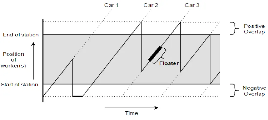
We now illustrate how overtime is caused, and how the position of the workers in a station changes over time (see Figure 14).

(29)

24

In Figure 14, the location of the worker(s) and time are displayed on the y- and x-axis respectively. At the start of every takt, a car enters the station, indicated by the diagonal dotted lines. These are the ‘paths’ the cars follow. Car 1 enters the station first, having a processing time smaller than the takt. The worker performs his activities on the car and then returns to the start of the station and waits for Car 2. The idle time is indicated with ‘A’ in Figure 14. Car 2 has a processing time longer than one takt, and the worker is finished the moment the car reaches the end of the positive overlap. He then moves back to the next car, and starts processing it at ‘B’. Notice that this is not the earliest starting time. As a result, Car 3 cannot be finished before reaching the end of the positive overlap, resulting in overtime indicated with ‘C’ in Figure 14.

4.2.4 Resolving overtime with floaters

To resolve the overtime that occurs in the assembly line, floaters are used. These cross-trained workers are deployed in the assembly line to resolve overtime by assisting regular workers at different stations. The function of floater is often occupied by the team leader of a part of the assembly line, but designated floaters are also used. It is assumed that floaters have the same productivity as regular workers, i.e., they can perform 52.8 seconds of processing time in one takt.

[image:29.595.74.522.338.539.2]

To illustrate how floaters resolve overtime, we give the following example. In Figure 14 we gave an example of overtime as a result from a car with a long processing time. Suppose we want to resolve the overtime on Car 3 (indicated with ‘C’ in Figure 14). In Figure 15 a floater is deployed to perform work on Car 3.

Figure 15. Effect of floater deployment

(30)

25

Figure 16. Station with overtime, original situation.

In Figure 17, the overtime is resolved by employing a floater on Car 3. The duration of stay of the floater is equal to the amount of overtime. This resolves the overtime on Car 3 but has no effect on the following car. In the original situation, the workers had to move back because the car reached the end of the overlap. In Figure 16, the workers still have to work until the car reaches the end of the overlap (with the difference that the activities on the car are completed).

Figure 17. Assistance on Car 3, overtime on Car 3 resolved.

Floater Allocation in Paced Mixed Model Assembly Lines: Design and implementation of a method for operational scheduling of cross trained workers in Mixed Model Assembly Lines

i