http://wrap.warwick.ac.uk
Original citation:
He, Ligang, Jarvis, Stephen A., 1970-, Spooner, Daniel P. and Nudd, G. R. (2003)
Dynamic scheduling of parallel real-time jobs by modelling spare capabilities in
heterogeneous clusters. In: IEEE International Conference on Cluster Computing, Hong
Kong, China, 01-04 Dec 2003. Published in: 2003 IEEE International Conference on
Cluster Computing, 2003. Proceedings. pp. 2-10.
Permanent WRAP url:
http://wrap.warwick.ac.uk/7668
Copyright and reuse:
The Warwick Research Archive Portal (WRAP) makes this work by researchers of the
University of Warwick available open access under the following conditions. Copyright ©
and all moral rights to the version of the paper presented here belong to the individual
author(s) and/or other copyright owners. To the extent reasonable and practicable the
material made available in WRAP has been checked for eligibility before being made
available.
Copies of full items can be used for personal research or study, educational, or not-for
profit purposes without prior permission or charge. Provided that the authors, title and
full bibliographic details are credited, a hyperlink and/or URL is given for the original
metadata page and the content is not changed in any way.
Publisher’s statement:
“© 2003 IEEE. Personal use of this material is permitted. Permission from IEEE must be
obtained for all other uses, in any current or future media, including reprinting
/republishing this material for advertising or promotional purposes, creating new
collective works, for resale or redistribution to servers or lists, or reuse of any
copyrighted component of this work in other works.”
A note on versions:
The version presented here may differ from the published version or, version of record, if
you wish to cite this item you are advised to consult the publisher’s version. Please see
the ‘permanent WRAP url’ above for details on accessing the published version and note
that access may require a subscription.
Dynamic Scheduling of Parallel Real-time Jobs by Modelling Spare Capabilities
in Heterogeneous Clusters
Ligang He, Stephen A. Jarvis, Daniel P. Spooner and Graham R. Nudd
Department of Computer Science, University of Warwick
Coventry, United Kingdom, CV4 7AL
{
liganghe, saj, dps, grn
}
@dcs.warwick.ac.uk
Abstract
In this research, a scenario is assumed where periodic real-time jobs are being run on a heterogeneous cluster of computers, and new aperiodic parallel real-time jobs, modelled by Directed Acyclic Graphs (DAG), arrive at the system dynamically. In the scheduling scheme pre-sented in this paper, a global scheduler situated within the cluster schedules new jobs onto the computers by modelling their spare capabilities left by existing periodic jobs. Admission control is introduced so that new jobs are rejected if their deadlines cannot be met under the pre-condition of still guaranteeing the real-time requirements of existing jobs. Each computer within the cluster houses a local scheduler, which uniformly schedules both peri-odic job instances and the subtasks in the parallel real-time jobs using an Early Deadline First policy. The mod-elling of the spare capabilities is optimal in the sense that once a new task starts running on a computer, it will util-ize all the spare capability left by the periodic real-time jobs and its finish time is the earliest possible. The per-formance of the proposed modelling approach and scheduling scheme is evaluated by extensive simulation; results show that the system utilization is significantly en-hanced, while the real-time requirements of the existing jobs remain guaranteed*.
1. Introduction
Cluster systems are gaining in popularity for process-ing scientific and commercial applications [6]. They are also increasingly used for processing applications with time constraints [1] as the work has been done to extend conventional operating systems, such as Linux, to support
*This work is sponsored in part by grants from the NASA AMES
Re-search Center (administrated by USARDSG, contract no. N68171-01-C-9012), the EPSRC (contract no. GR/R47424/01) and the EPSRC e-Science Core Programme (contract no. GR/S03058/01).
real-time scheduling (for example, the preemptive sched-uling based on the Earliest-Deadline-First policy) [5][16]. Real-time processing can often be represented abstractly as the hybrid execution of existing periodic jobs together with newly arriving aperiodic jobs. An example of this is in the reservation-based scheduling of multimedia appli-cations, where the reservation of processor times can be expressed per period, so as to ensure that the processor utilization for an application is maintained above a de-sired level [9]. These reserved executions can be viewed as periodic jobs and besides the reserved executions, the processors have also to deal with other newly arriving jobs. This scenario presents the challenge of devising scheduling schemes which judicially deal with the hybrid execution of existing jobs (or reserved executions) to-gether with newly arriving jobs. This task is complicated when the objective is to reduce the response times of newly arriving jobs while maintaining the time con-straints of existing periodic jobs.
The dynamic scheduling technique presented in this paper addresses this issue, aiming to allocate newly arriv-ing Aperiodic Real-time Jobs (ARJ) to a heterogeneous cluster of computers on which Periodic Real-time Jobs
in-stances and the tasks in the ARJs so as to reduce the local scheduling complexity.
The approach for modelling spare capabilities pro-posed in this paper does not invoke any communication overhead between the global scheduler and the remaining computers in the cluster. The approach is optimal in the sense that once a new task starts running, it will utilize all the spare capability left by the PRJs, and its finish time is the earliest possible.
The rest of the paper is organized as follows. Section 2 presents related work. Section 3 describes the workload and system model. In section 4, a novel approach is pre-sented to enable the global scheduler to model spare ca-pabilities of computers in a cluster. Section 5 proposes a global dynamic scheduling algorithm for parallel real-time jobs. The performance evaluation is presented in Section 6 and Section 7 concludes the paper.
2. Related work
Studies on heterogeneous clusters or networks of workstations have received a good deal attention [7][17]. The scheduling of tasks with precedence constraints, which are usually represented by Directed Acyclic Graphs (DAG), has also been documented in a number of papers [2][11][19][20]. An off-line algorithm is presented in [2] to schedule communicating tasks with precedence constraints in distributed systems. However, the algorithm belongs to the static category. Paper [20] describes a run-time incremental DAG scheduling approach on parallel machines. The approach is however limited to homoge-nous systems. Two low-complexity heuristics, the Het-erogeneous Earliest-Finish-Time Algorithm and the Criti-cal-Path-on-a-Processor Algorithm are proposed in [19] for scheduling DAGs on heterogeneous processors. How-ever, the heuristics are designed for non-retime task al-location. In [11] non-real-time DAGs are extended to in-clude real-time information, and the scheduling of parallel tasks with real-time DAG topologies onto heterogeneous systems is proposed. This technique however is not aimed at using spare system capabilities. The scheduling scheme presented in this paper dynamically schedules parallel real-time jobs with real-time DAGs on heterogeneous clusters. Both task scheduling and message scheduling are taken in account in the algorithm design.
A number of scheduling algorithms for periodic real-time jobs on multi-computer or multiprocessor systems have also been presented [3][12]. A task duplication tech-nique combined with pipelined execution is presented in [12], allowing the scheduling of time critical periodic ap-plications on heterogeneous systems. [3] addresses the reward-based scheduling problem for periodic tasks, which assumes that a periodic task comprises a manda-tory and an optional part. While these techniques are
ef-fective, they are unable to deal with the hybrid execution of periodic and aperiodic tasks.
Scheduling systems for processing both periodic and aperiodic real-time tasks can be classified into fixed or dynamic priority systems. Dynamic priority systems typi-cally attain higher processor utilization than fixed ones. Slack Stealing policies have been designed for fixed pri-ority systems [8] while the Background (BG), Deadline Deferrable Server (DDS), Total Bandwidth Server (TBS) and Improved Priority Exchange (IPE) algorithms have been designed for dynamic priority systems [4][13][15]. These techniques are widely used in embedded real-time systems, such as robot control systems. All these algo-rithms have been developed for uniprocessor architectures and aperiodic tasks are assumed independent without precedence constraints. The techniques presented in [8] and [18] run aperiodic tasks by using the spare capability left by periodic tasks. Unfortunately, such schemes are limited to uniprocessor scenarios.
It is a non-trivial task to extend the modelling of spare capability from uniprocessor architectures to cluster envi-ronments. A uniprocessor system only models the spare capability in itself. In a cluster scenario however, a cen-tral node models the spare capabilities of other nodes, so the information needed for calculating spare capabilities is far more difficult to attain. An efficient modelling ap-proach for clusters that avoids significant communication overheads among nodes is therefore needed. The model-ling approach in this paper is able to model spare capabil-ity of computers in a heterogeneous cluster and is free of additional communication overheads. The scheme in this paper is also designed for dynamic priority systems and an EDF policy is used in the local scheduling.
3. Workload and system model
A heterogeneous cluster of computers is modeled as
P={p1, p2,..., pm}, where piis an autonomous computer. Each computer pi is weighted pwi, which represents the time it takes to perform one unit of computation. The computers in the heterogeneous cluster are connected by a multi-bandwidth local network. Each communication link between computer pi and pj, denoted by lij, is weighted
lwij, which models the time it takes to transfer one unit of message between pi and pj.
Each computer runs a set of PRJs, all of which are in-dependent of one another. On a computer with n PRJs, the
i-th periodic real-time job PRJi (1≤i≤n) is defined as (Si,
must meet their deadlines and are scheduled using an EDF policy. Fig.1 shows two PRJs and their execution on a single computer; all the illustrations in this paper use these two PRJs as a working example.
PRJ1
0 2 4 6 8 10 12 PRJ11 12 13
0 2 4 6 8 10 12
PRJ21 22 23 24 PRJ2
0 2 4 6 8 10 12 2212 231324
PRJ2111
[image:4.595.62.286.153.251.2](a) (b) (c)
Figure 1.A case study of PRJs (a) PRJ1 with a
pe-riod of 4 and an execution time of 1, (b) PRJ2 with a period of 3 and an execution time of 1, (c) execution of PRJ1 and PRJ2 under EDF
ARJs arrive at the heterogeneous cluster dynamically. If accepted, an ARJ is run once. An ARJ is modeled as (avt, J), where avt is the ARJ’s arrival time and J defines the tasks and their topology in the ARJ. J={V, E}, where
V={v1, v2,…, vr}, which defines r real-time tasks that con-stitute the ARJ. dt(vi) and cvi are denoted as vi’s deadline and computational volume; E represents the communica-tion relacommunica-tionship and the precedence constraints among tasks; eij=(vi, vj)∈E represents a message sent from task vi to vj and it also suggests vj can start running only after vi is complete and vj receives message eij; vi is called vj’s predecessor and mvij is denoted as message eij’s volume.
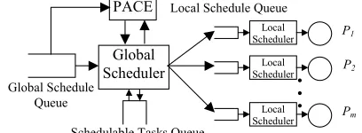
Fig.2 depicts the components of the scheduler model in the heterogeneous cluster environment. It is assumed that PRJs are active across the constituent computers, and a central computer in the cluster, the global scheduler, re-cords Si, Ci and Ti of all PRJs. The global scheduler mod-els the cluster spare capacities left by the PRJs.
Schedulable Tasks Queue Global Schedule
Queue
• • • Global
Scheduler
Pm
P2
P1
Local Schedule Queue
Local Scheduler
Local Scheduler
[image:4.595.314.533.435.624.2]Local Scheduler PACE
Figure 2.The scheduler model in the
heterogene-ous cluster environment
When the global scheduler fetches a newly arriving ARJ from the head of the global schedule queue, it inserts the schedulable tasks in the ARJ into the schedulable task queue. The global scheduler then picks a task from the head of the schedulable task queue and schedules it glob-ally. Once an ARJ is accepted, tasks in the ARJ are sent to the local schedulers of the designated computers. At each computer, the local scheduler uniformly schedules both the ARJs’ tasks and the PRJs’ PJIs using EDF. The local schedule is preemptive.
PACE is a performance prediction toolkit [10]. In this scheduler model, PACE accepts ARJs, predicts the execu-tion time of each task in the ARJs on each computer and returns the predicted time to the global scheduler. After the global scheduler decides to schedule task vi on
com-puter ps, assuming message eij=(vi, vj)∈E, PACE is called to predict eij’s communication time on each link between
ps and any other computer. The efficiency of the PACE evaluation engine enables the real-time production of per-formance data [14].
4. Spare capability modelling
In this section, the initial distribution of idle time left by the PRJs running on the computers is modelled. The idle time distribution will be altered by the dynamic arri-vals of ARJs. Hence, an on-line mechanism is presented for adjusting the initial idle time distribution when the global scheduler schedules a newly arriving ARJ.
4.1. Off-line modelling of the initial distribution
of spare capabilities
As an example, consider the two PRJs found in Fig.1 that are mapped to a single computer. Consider the case for PRJ1 where there are 4 time units before PJI11’s
dead-line and there are two tasks, PJI11 and PJI21, which must be completed before that time. There are therefore 2 idle time units before PJI11’s deadline. In the case of PRJ2 there are 6 time units before PRJ22’s deadline and 3 tasks,
PJI11, PJI21 and PJI22, which must be completed before that time. In this case, 3 idle time units are available be-fore the deadline.
S1(t) 2
5 4
0 4 8 12
S2(t)
5 2
4 3
0 4 8 12 (a) (b)
S(t)
5 4 3 2
0 4 8 12 0 4 8 12
PRJ
21 11 22 122313 24New t ask
(c) (d)
Figure 3. A case study of the function of idle time
units (a) Function of idle time units for PRJ1 (b) Function of idle time units for PRJ2 (c) Function of idle time units for both PRJ1 and PRJ2 (d) The joint execution of PRJ1, PRJ2 and a new task with an execution time of 4 starting at 0
The above calculation can be performed for all PJIs of any PRJi running on the same computer, and a function constructed of idle time units corresponding to PRJi, de-noted as Si(t), is defined in Eq.1, where Dij is PJIij’s dead-line (let Di0 be 0), Pij is the sum of execution time of PJIs that must be completed before Dij.
Si(t)= Dij-Pij Di(j-1)<t≤Dij, 1≤ i≤n, j≥1 (1)
[image:4.595.68.272.456.531.2]
∑
= = n k k kij T C
P
1
* /
α , where,
k ij k ij k ij S D S D S D ≤ > − = 0
α (2)
Fig.3.a and Fig.3.b show the functions of idle time units within a certain time period, S1(t) and S2(t), corre-sponding to PRJ1 and PRJ2 in Fig.1 respectively. In the figures, the time points, except zero, at which the function value increases, are called Jumping Time Points (JTP). A
JTP is a PJI’s deadline. In Fig.3.a, the JTPs are 4 and 8. If the number of time units that are used to run new tasks between time 0 and any JTP is less than Si(JTP), the deadlines of all PJIs of PRJi can be guaranteed.
Suppose n PRJs (PRJ1,..., PRJi,..., PRJn) are running on a single computer, then the distribution function of idle time left by the PRJs, denoted as S(t), can be derived from the individual Si(t) (1≤i≤n). For any time t, S(t) obtains its value from the minimum of all Si(t), shown in Eq.3.
S(t)=min{Si(t)|1≤i≤n} (3)
JTPs are also defined in S(t), as with Si(t). S(t) suggests that idle time units of S(JTP) are available in [0, JTP]. Thus, in order to satisfy the real-time requirements of all PRJs, for any JTP, at most S(JTP) time units can be used to run new tasks in [0, JTP]. The initial distribution of spare capabilities in each computer is constructed off-line.
S(t) corresponding to the PRJ set consisting of PRJ1 and PRJ2, is plotted in Fig. 3.c. Fig.3.d illustrates the exe-cution of a new task in which the real-time requirements of PRJ1 and PRJ2 is still guaranteed. The execution coin-cides with function S(t) in Fig.3.c, that is, between time 0 and any JTP there are exactly S(JTP) time units used to run the new task.
4.2. On-line modelling of the spare capability
distribution
If a new task starts running at any time t0, the number
of idle time units in [t0, JTP] (t0<JTP), denoted by S(t0, JTP), needs to be calculated on-line. In order to do this, it is necessary to calculate the proportion of workload that all PJIs which are to complete in [0, JTP] have finished before t0, and also how much finishes in [t0, JTP]. The
remaining time in [t0, JTP] will then be spare. This
calcu-lation involves identifying what PJIs must be complete before t0, and what PJIs can start before t0 but must be
complete before the JTP. Some notation is introduced be-low to classify the PJIs.
PJ(t0) is a set of PJIs whose deadlines are no more than
time t0. Hence, all PJIs in PJ(t0) must be complete before t0. PJ(t0) is defined in Eq.4.
PJ(t0)={PJIij| Dij≤t0} (4) P(t0) are denoted as the number of time units in [0, t0]
that are used for running the PJIs in PJ(t0). P(t0) can be
calculated by Eq.5.
∑
= = n k k k C T t P 10) / *
( α , where,
k k k S t S t S t ≤ > − = 0 0 0 0
α (5)
Let JTP1, JTP2,..., JTPk be a sequence of JTPs after t0
in the spare capability distribution function S(t) and JTP1
the nearest to t0. LJk(t0) is a set of PJIs, whose ready times
are less than t0, and whose deadlines are more than t0 but
no more than JTPk. LJk(t0) is defined in Eq.6. All PJIs in LJk(t0) can start running before t0 but must be complete
before JTPk. Lk(t0) is denoted as the number of time units
in [0, t0] that are used to run the PJIs in LJk(t0).
LJk(t0)={ PJIij | Rij<t0<Dij and Dij≤JTPk} (6) In Theorem 1, S(t0, JTPk) is related to S(JTPk). S(JTPk)
is obtained directly from the initial spare capability distri-bution function established off-line in subsection 4.1.
Theorem 1. Suppose t0 is any time point in [0, JTPk],
then S(JTPk) and S(t0, JTPk) satisfy the following equation: S(t0, JTPk)=S(JTPk)−t0+P(t0)+Lk(t0) (7)
Proof: PJIs whose deadlines are less than JTPk must be completed in [0, JTPk]. Their total workload is P(JTPk) (see Eq.5). The workload of P(t0) and Lk(t0) has to been
finished before t0, so the workload of P(JTPk)−P(t0)−
L
k(
t
0)
must be done in [t0, JTPk]. Hence, the maximal number of
time units that can be spared to run new tasks in [t0, JTPk],
i.e. S(t0,JTPk), is (JTPk-t0)−(P(JTPk)−P(t0)−Lk(t0)). Thus,
the following equation exists:
S(t0,JTPk)=JTPk−P(JTPk)−t0+P(t0)+Lk(t0)
In addition, JTPk−P(JTPk)=S(JTPk). Hence Eq.7 holds.
Lk(t0) in Eq.7 still remains unknown. The rest of the
subsection documents the calculation of Lk(t0).
If there are new tasks running before t0, the execution
process of PJIs in PJ(t0) may change so that they may not
retain the same execution pattern as the case when PRJs alone are executing. Theorem 2 is introduced to reveal the distribution property of the remaining time units before t0
after running PJIs in PJ(t0) as well as the new tasks.
Theorem 2. Suppose the last executed new task is com-pleted at time f, then there exists such a time point ts in [f,
t0] (t0>f), where
1. either PJIs in PJ(t0) retain the same execution
pat-tern in [ts, t0] as the case when no new tasks are run
be-fore t0, or all PJIs in PJ(t0) are completed before ts,
2. there are no idle time slots in [f, ts],
3. ts can be determined by Eq.8, where
I
tp0(
t
s,
t
0)
repre-sents the number of time units left in [ts, t0] after
execut-ing PJIs in PJ(t0); ,
(
,
0)
0
t
f
I
tA
P represents the number of time
units left in [f, t0] after executing both PJIs in PJ(t0) and
also the new tasks.
)
,
(
)
,
(
0 0, 00
t
t
I
f
t
I
tA P s
t
p
=
(8)Proof: The execution of the last new tasks may delay the execution of PJIs in PJ(t0). The delayed PJIs may also
de-lay other PJIs in PJ(t0) further. The delay chain will
PJ(t0) must be complete before t0, such a time point, ts,
must exist that satisfies Theorem 2.1. Since there are un-finished workloads before ts, Theorem 2.2 also exists. Eq.8 is a direct derivation from Theorem 2.1 and 2.2.
Theorem 2 is illustrated by comparing the PJIs’ execu-tion in Fig.1.c and 3.d. In Fig.1.c, PJI12 and PJI23 finish at time 5 and 7 respectively. Due to the execution of the new task, PJI12 and PJI23 are delayed to finish at times 8 and 9, respectively, shown in Fig.3.d. PJI23’s delay, further de-lays PJI13, and PJI24 is then delayed by PJI13. In Fig.3.d however, PJIs ready after time 11 can be run without fur-ther disruption. Time 11 can be set as ts in the example.
As shown in Theorem 2, PJIs in PJ(t0) running in [ts, t0]
retain the original execution pattern (as though there were no preceding new tasks). Hence the remaining time units in [ts, t0] after running these PJIs can be calculated; these
time units can only be occupied by PJIs in LJk(t0).
Conse-quently, Lk(t0) in Eq.7 can be calculated. The algorithm
for computing Lk(t0) is omitted in this paper.
5. Scheduling algorithm
Let vi be a task in an ARJ. Denote stk(vi) and ftk(vi) as task vi’s earliest possible start time and its finish time on computer pk. It is assumed that tasks vi1, vi2,…, viq(viq is the last task) have been scheduled on pk. stk(vi) can be cal-culated using Eq.9, where, mltk(vi) is the latest time when all messages from vi’s predecessors arrive at pk.
otherwise rs predecesso has v v ft avt v ft v mlt v st i iq k iq k i k i k = )) ( , max( )) ( ), ( max( )
( (9)
Suppose vi is scheduled on computer pk. The arrival time of the message from vi’s predecessor vj to vi (i.e. message eji) is denoted by matk(vj, vi). If vj is also sched-uled on pk, then matk(vj, vi) equals ftk(vj). Suppose vj is scheduled on ps (s≠k) and there exists a message schedule sequence, (mstsk
1 ,mft1sk), (
sk mst2 ,
sk
mft2 ),…, (mstask, sk a
mft ), in the communication link between ps and pk, where
sk i
mst and
mft
iskare the starting time and finish time of a message transferring in the communication link; then the first idle time slot in the communication link satisfying Eq.10 is used to send eji, where comsk(eji) is the communi-cation time of eji in the communication link between ps and pk; this idle slot is supposed to be ( skb
mft , sk
b
mst +1).
sk q
mst -max( sk q
mft
−1, fts(vj))≥ comsk(eji) (1≤q≤a+1, letsk
mft
0 =0,mst
ask+1=∞) (10)Thus, matk(vj, vi) can be calculated by Eq.11.
k s k s v ft e com v ft mft v v mat j k ji sk j s b i j k = ≠ + = ) ( ) ( )) ( , max( ) ,
( (11)
Then, mltk(vi) in Eq.9 can be calculated by Eq.12.
mltk(vi)=max{matk(v
j, vi)| vj is vi’s predecessor} (12)
The complete scheduling procedure for ARJs is as fol-lows. The global scheduler fetches an ARJ from the head of the global schedule queue, and inserts the schedulable tasks in the ARJ (a task is schedulable if it either has no predecessors or all of its predecessors have been sched-uled) into the schedulable task queue so that the deadlines of the tasks are in increasing order. The global scheduler then picks a task from the head of the queue and sched-ules it globally. The starting time of a task vi is calculated as Eq.9. Suppose that vi starts at t0 on computer pj, using
Eq.7, the global scheduler can calculate in pj how many idle time units there are between t0 and any JTP following t0, which can be used to run vi. Therefore, it can be
deter-mined before which JTP vi can be completed. Conse-quently, vi’s finish time at any computer can be deter-mined. This is shown in Algorithm 1.
Algorithm 1. Calculating the finish time of task vi
starting at t0 in computer pj
1. cj(cvi)← vi’s execution time on pj (predicted by PACE); 2. Calculate P(t0) using Eq.5; Get ts using Eq.8;
3. Get the first JTP after t0;
4. Call Algorithm 1 to calculate the corresponding Lk(t0);
5. Calculate S(t0, JTP) using Eq.7;
6. while (S(t0, JTP)<cj(cvi))
7. OJTP←JTP;Get the next JTP; 8. Calculate S(t0, JTP) by Eq.7;
9. end while
10.ftj(vi)←OJTP+cj(cvi)-S(t
0, OJTP);
If vi’s finish time on any computer in the cluster is greater than its deadline, the ARJ that vi belongs to is re-jected. The admission control is shown in Algorithm 2.
Algorithm 2. Admission Control
1. PC←Φ;
2. for each computer pj in the cluster do
3. Calculate vi’s starting time on pj, stj(vi), using Eq.9; 4. Call Algorithm 1 to calculate vi’s finish time on pj,
ftj(vi);
5. if (ftj(vi)≤dt(vi)) then 6. PC=PC∪{pj}; 7. end for
8. if PC=Φthen reject vi and the ARJ that vi belongs to; 9. else accept vi;
When vi’s deadline can be met in more than one com-puter, two possible Second-level Selection Policies are of-fered to choose a final computer. One is a Response First
(RF) policy, which selects the computer on which vi has the earliest finish time. The other is Utilization First (UF) policy, which selects the computer on which vi has the longest execution time. The two policies have different selection inclinations. In section 6 the performance of these two policies is evaluated.
When the local scheduler in any computer receives the allocated ARJs’ tasks or the PJIs of the PRJs are ready, it inserts them into the Local Schedule Queue ordered in in-creasing deadlines. A local scheduler fetches a task (ARJ’s task or PJI) from the head of the queue and the task is then executed. Once the task with the lower dead-line is ready, the current execution is preempted.
Assume that the initial distribution of spare capabilities on each computer in the heterogeneous cluster is con-structed off-line. The on-line global dynamic scheduling algorithm (GDS) is shown in Algorithm 3.
Algorithm 3. Global dynamic scheduling for parallel real-time jobs
1. if global scheduler queue=Φthen wait until a new ARJ arrives, then go to step 3;
2. else
3. Get a job from the head of global scheduler queue and insert its schedulable tasks into the schedulable task queue;
4. for each task vi in the schedulable task queue do
5. Call Algorithm 2 to exert admission control; 6. if accept vi then
7. Call a second-level selection policy to choose a computer pj;
8. Reset vi’s deadline to be its computed finish time
ftj(vi);
9. Search for new schedulable tasks in the ARJ and insert them into the schedulable task queue; 10. else go to step 1;
11. end if
12. end for
13. Dispatch the tasks in the ARJ to designated computers; go to step 1;
14.end if
Since vi’s deadline is reset to its finish time, vi will be forced to run between its starting time and the deadline. As the modelling analysis suggests in Section 4, vi cannot be finished earlier on the computer on which it is sched-uled. Otherwise, the deadlines of some PJIs on that com-puter must be missed. In this sense, the modelling ap-proach is optimal. When the global scheduler models spare capacities in other computers, no information has to be transferred among them in order to make scheduling decisions. Hence no communication overhead is incurred by the modelling approach.
6. Performance evaluation
The experimental parameters in our simulation studies are chosen either based on those used in the literature [8][11] or to represent a realistic workload.
Sets of 40 PRJs are randomly generated with periods ranging from 42 to 15015. The level of PRJ workloads (PLOAD) is set by varying PRJs’ execution times. Three
levels of PLOAD, light, medium and heavy, are generated for each computer, which provides 10%, 40% and 70% system utilization, respectively.
In the simulation, task vi’s execution time on computer
pj is calculated as cvi*pwj; similarly, message eij’s communication time on link lst is mvij*lwst. In a hetero-geneous cluster, computer pi’s weight pwi is uniformly chosen between MIN_PW and MAX_PW. This range re-flects the level of computational heterogeneity. The weight of a communication link is uniformly chosen be-tween MIN_LW and MAX_LW. This range reflects the level of communication heterogeneity.
Each point in the performance curve is plotted as the average value of the corresponding performance measure of 10,000 independent ARJs. ARJs are assumed to arrive following a Poisson process with an arrival rate λ. Each ARJ has a randomly generated DAG topology with a given number of tasks (TASKNUM); task vi’s computa-tional volume cvi is uniformly chosen between MIN_CV
and MAX_CV and the volume of a message among tasks is uniformly chosen between MIN_ MV and MAX_MV.
vi’s deadline is defined as follows: if vi has no predeces-sors in the DAG, dt(vi)=avt+cvi*nw*(dr+1), where the parameter dr is uniformly chosen between MIN_DR and
MAX_DR, and
nw
is the geometric mean of the weight of all computers; otherwise, [image:7.595.312.534.443.651.2]dt(vi)=max{dt(vj)}+cvi* nw*(dr+1) where vj is vi’s predecessor.
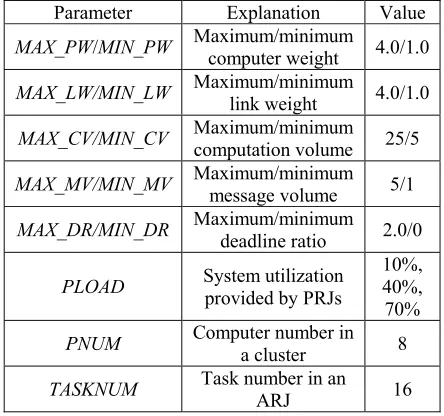
Table 1 Parameters for simulation studies
Parameter Explanation Value
MAX_PW/MIN_PW Maximum/minimum
computer weight 4.0/1.0
MAX_LW/MIN_LW Maximum/minimum link weight 4.0/1.0
MAX_CV/MIN_CV Maximum/minimum computation volume 25/5
MAX_MV/MIN_MV Maximum/minimum
message volume 5/1
MAX_DR/MIN_DR Maximum/minimum deadline ratio 2.0/0
PLOAD System utilization
provided by PRJs
10%, 40%, 70%
PNUM Computer number in a cluster 8
TASKNUM Task number in an ARJ 16
The values of the simulation parameters are given in Table 1 unless otherwise stated. Three metrics are meas-ured in the simulation experiments: Guarantee Ratio
defined as the fraction of busy time for running tasks to the total time available in the cluster. An ARJ’s response time is defined as the difference between its arrival time and the finish time of the last task to be run. RT is the av-erage response time for all ARJs.
6.1. Job workloads and second-level selection
policies
RT can be viewed as a measure of the capability of the scheme in utilizing the spare capability in the computers. Fig.4.a compares the global dynamic scheduling algo-rithm (GDS) presented in this paper in terms of RT with four other algorithms for dynamic priority systems in the literature [4][13][15], i.e. Background (BG), Deadline Deferrable Server (DDS), Total Bandwidth Server (TBS) and Improved Priority Exchange (IPE). It is noted that our GDS algorithm is devised for scheduling parallel real-time jobs in a cluster scenario, but all other algorithms are designed for scheduling periodic and independent aperi-odic tasks (non-parallel tasks) in uniprocessor architec-tures. In order to make a fair comparison, in this experi-ment the GDS is downgraded to schedule independent real-time tasks in a cluster of two computers, one acting as the global scheduler, the other housing a local sched-uler and jointly running tasks; the computational volumes of tasks follow the exponential distribution. To stress the response performance, the GR of non-periodic real-time tasks is fixed to be 1.0 by assigning extremely loose dead-lines. An M/M/1 queuing model is used to compute the ideal bound for RT of the same workload but in the ab-sence of PRJs.
5 15 25 35
2 3 4 5 6 7 8 9 10 arrival rate(10-2)
RT BG
DDS TBS IPE GDS M/M/1
100 150 200 250 300 350 400
6 10 14 18 22 26 30
arrival rate(10-3)
RT 70% PRJ 40% PRJ 10% PRJ no PRJ
(a) (b)
Figure 4.(a) Comparison of RT among the
down-graded GDS, other traditional algorithms and an
M/M/1 queuing model; PLOAD=40%, the average
computational volume of tasks is 8, the com-puter weight is 1.0 (b) Comparison between the GDS and the ideal bound (no PRJ); RF policy MAX_CV/MIN_CV=12/4
As can be observed from Fig.4.a, the GDS outperforms other algorithms and shows the same performance as the M/M/1 queuing model except the arrival rate λ is greater than 0.08. The results coincide with the conclusion in Section 5, i.e. our algorithm is optimal in exploiting spare
capabilities in a computer. Fig.4.b displays under the Re-sponse-First policy, the RT of parallel real-time jobs as a function of λ in a heterogeneous cluster of 8 computers under different levels of PLOAD. An ideal bound of RT is generated for comparison by running the same ARJ work-loads in the same heterogeneous cluster in the absence of PRJs. The GR of the ARJs is also fixed to be 1.0. It is ob-served from Fig.4.b that in the case of 10% PLOAD, the RT obtained by the GDS is very close to the ideal bound, indicating the excellent performance of the GDS in utiliz-ing spare capabilities to schedule parallel real-time jobs in a cluster scenario.
20 40 60 80 100
4 6 8 10 12 14 16 18 20 22 arrival-rate(10-3
) GR(%)
20 40 60 80 100
4 6 8 10 12 14 16 18 20 22 arrival-rate(10-3)
SU(%)
(10%,RF) (10%,UF) (40%,RF) (40%,UF) (70%,RF) (70%,UF)
[image:8.595.312.534.248.373.2](a) (b)
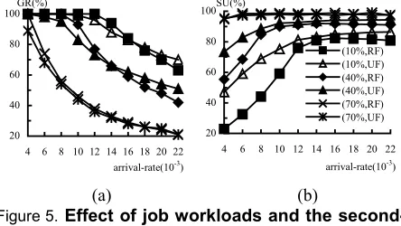
Figure 5. Effect of job workloads and the
second-level selection policies on (a) GR (b) SU; Leg-ends for Fig.5.a are the same as those in Fig.5.b
Fig.5.a and b display the metrics GR and SU as the function of λ under the second-level selection policies of the Response-First and the Utilization-First, respectively. The first observation from Fig.5.a is that the GR de-creases as λ increases in all cases, as expected. A further observation is that in the case of 10% and 40% PLOAD, the RF policy outperforms the UF when λ is low, while when λ exceeds a threshold, the opposite is true. This may be because that the RF policy is predisposed to first choose the better computers, whereas UF has the opposite trait. The experimental results suggest that when the ARJ workload is so high that all the computers in a heteroge-neous cluster will be heavily occupied, allocating work-load to poorer nodes and then to better nodes is more ap-propriate than allocating in the opposite direction.
contrib-utes more to the improvement of SU than the RF policy. The experimental results suggest that utilization of the cluster is significantly enhanced compared with the origi-nal PLOAD.
6.2. Computation and communication
heteroge-neity
Fig.6.a shows the impact of computational heterogene-ity on the metrics GR and SU. Fig.6.b and Fig.6.c show the impact of communicational heterogeneity on GR and SU, respectively, under different levels of the computa-tional heterogeneity. Only the results for 40% PLOAD
and the RF policy are shown as the results for the other cases demonstrate similar patterns.
20 40 60 80 100
[5,5] [4,6] [3,7] [2,8] [1,9]
Computational heterogenity
GR(%) SU(%)
70 76 82 88 94 100
[5,5] [4,6] [3,7] [2,8] [1,9] Communication heterogeneity SU(%) CPH=[5,5]
CPH=[3,7] CPH=[1,9]
(a) (b)
40 50 60 70 80 90 100
[5,5] [4,6] [3,7] [2,8] [1,9] Communication heterogeneity GR(%)
CPH=[5,5] CPH=[3,7] CPH=[1,9]
(c)
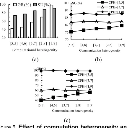
Figure 6. Effect of computation heterogeneity and
communication heterogeneity, the RF policy and PLOAD=40% (a) Effect of computational hetero-geneity on GR and SU, λ=0.006 (b) Effect of the communication heterogeneity on SU, λ=0.006 (c) Effect of the communication heterogeneity on GR, λ=0.006
The levels of computation and communication hetero-geneity are measured by the scale of the range from which computer weights and communication link weights are selected. Five sets of computer and link weights, all with the same average, are uniformly chosen from five ranges, [1,9], [2,8], [3,7], [4,6] and [5,5].
As can be observed from Fig.6.a, GR and SU improve as the computational heterogeneity increases. The in-crease in GR may be because as the computation hetero-geneity increases, the increasing variance in a task’s exe-cution time provides the task with more chance of fitting into the idle time slots before its deadline in the cluster. Under the same workloads, the increase in GR leads to an
increase in SU. It can be observed from Fig.6.b and Fig.6.c that SU and GR increase as the communication heterogeneity increases in the case when the computation heterogeneity is [5,5] (i.e. homogeneity). This may be be-cause the increasing variance in message transfer time provides more chance of finding a suitable idle time slot in the communication channels. However, the communi-cation heterogeneity has no obvious impact on SU and GR when the computation heterogeneity increases to [3,7] or [1,9]. This suggests that the level of computation het-erogeneity is more critical for scheduling ARJs than the level of the communication heterogeneity.
6.3 Task size and message size
Fig.7.a shows the impact of the size of tasks in ARJs on GR and SU. Only the results for 40% PLOAD are shown; the results for the other levels of PLOAD show similar patterns. The task size is measured by the average computational volume of tasks in an ARJ. In this experi-ment, when the task size increases, the average arrival rate λ is set to decrease proportionally so as to keep the total ARJ workload unchanged.
60 70 80 90 100
5 10 15 20 25 30 Task size
(GR,RF) (SU,RF) (GR,UF) (SU,UF)
20 40 60 80 100
15/3 12/6 9/9 6/12 3/15
T ask size/Message size
GR(%) SU(%)
[image:9.595.65.280.284.501.2](a) (b)
Figure 7. Effect of task and message size,
PLOAD=40% (a) Effect of task size on GR and SU,
λ is 0.025 when the task size is 5 (b) Effect of task-size/message-size ratio on GR and SU,
λ=0.02, RF
[image:9.595.313.538.371.547.2]Fig.7.b demonstrates the effect, on GR and SU, of the ratio of the task size to the size of messages among tasks. Only the results for 40% PLOAD and the RF policy are presented since other cases have similar behaviours. The message size of an ARJ is measured by the average vol-ume of all messages among tasks in the ARJ. The task-size/message-size ratio varies from 15/3 to 3/15, all with the same volume sum. As can be observed from Fig.7.b, the impact of the task-size/message-size ratio is also mixed. GR improves but SU decreases as the task-size/message-size ratio increases. The increase in GR can be explained as follows. First, it is easier for small tasks to be admitted as demonstrated above. Second, although the message size increases as the task-size/message-size ratio decreases, the scheduling policy may compensate for this by scheduling two tasks on the same computer if the communication time between them is too long. Finally, computers are shared by ARJs and PRJs, while communi-cation links are exclusively utilized by ARJs. These re-sults indicate that in an ARJ, the task size is a more criti-cal parameter than the message size for the ARJ’s admis-sion and response time.
7. Conclusions
In this paper a scheduling framework is presented to schedule dynamic aperiodic parallel real time jobs by modelling spare capabilities of a heterogeneous cluster on which periodic real-time jobs are running. The approach of spare-capability modelling is optimal in the sense that once a new task starts running, it will utilize all spare ca-pability and its finish time is the earliest possible. No communication overheads are incurred by this approach. Scheduling for ARJs takes both task and message sched-uling into account. Extensive simulations are conducted that show that system utilization is significantly enhanced without impacting on the QoS of existing jobs. Future studies are planed to extend the scheduling scheme to take the prediction, scheduling and dispatch time of ARJs into account.
8. References
[1] M. Apte,S. Chakravarthi,J. Padmanabhan andA. Skiellum, “A Synchronized Real-Time Linux Based Myrinet Cluster for Deterministic High Performance Computing and MPI/RT,” The
15th International Parallel and Distributed Processing
Sympo-sium, 2001.
[2] T. F. Abdelzaher, K. G. Shin,“Combined Task and Message Scheduling in Distributed Real-Time Systems,”IEEE
Transac-tions on parallel and distributed systems, 10(11), November
1999.
[3] H. Aydin, R. Melhem, D. Mosse, and P. Mejia-Alvarez, “Optimal reward-based scheduling of periodic real-time tasks,”
The 20th IEEE Real-Time Systems Symposium, December 1999.
[4] M. Caccamo, G. Lipari, and G. Buttazzo, “Sharing Re-sources with the TB* Server,” IEEE Real-Time Systems Sympo-sium, 1999.
[5] D. B. Golub, “Operating System Support for Coexistence of Real-Time and Conventional Scheduling,” The 1st Symposium
on Operating Systems Design and Implementation, 1994.
[6] K. Hwang and Z. Xu, Scalable Parallel Computing: Tech-nology, Architecture, Programming. McGraw Hill, 1998. [7] D. Kebbal, E.G. Talbi, J.M. Geib, “Building and Scheduling Parallel Adaptive Applications in Heterogeneous Environ-ments,” 1st IEEE Computer Society International Workshop on
Cluster Computing, December, 1999.
[8] J. P. Lehoczky and S. Ramos-Thuel, “An Optimal Algorithm for Scheduling Soft-Aperiodic Tasks in Fixed-Priority Preemp-tive Systems,” Proc. of Real-Time Systems Symposium, 1992, pp.110-123.
[9] C.W. Mercer, S. Savage, and H. Tokuda, “Processor Capac-ity Reserves: Operating System Support for Multimedia Appli-cations,” Proc of the IEEE International Conference on Multi-media Computing and Systems, 1994.
[10] G.R. Nudd, D.J.Kerbyson et al, “PACE-a toolset for the performance prediction of parallel and distributed systems,” Intl Journal of High Performance Computing Applications, Special
Issues on Performance Modelling, 14(3), 2000, 228-251.
[11] X. Qin and H. Jiang, “Dynamic, Reliability-driven Scheduling of Parallel Real-time Jobs in Heterogeneous Sys-tems,” The 30th International Conference on Parallel
Processing, Valencia, Spain, September 3-7, 2001.
[12] S. Ranaweera, and D. P. Agrawal, “Scheduling of Periodic Time Critical Applications for Pipelined Execution on Hetero-geneous Systems,” Proceedings of the 2001 International
Con-ference on Parallel Processing, 2001.
[13] D A. E Salaheddine, “Aperiodic Scheduling in a Dynamic Real-Time Manufacturing System,” IEEE Real-Time Embedded
System Workshop, 2001.
[14] D. P. Spooner, S. A. Jarvis, J. Cao, S. Saini and GR. Nudd, “Local Grid Scheduling Techniques using Performance Predic-tion,” IEE Proc-Computers and Digital Techniques, 150(2): 87-96, 2003.
[15] M. Spuri and G. Buttazzo, “Scheduling Aperiodic Tasks in Dynamic Priority Systems,” Real-Time Systems 10(2), 1996, 179-210.
[16] B. Srinivasan, S. Pather, F. Ansari, and D. Niehaus, “A Firm Real-Time System Implementation Using Commercial Off-The-Shelf Hardware and Free Software,” The 4th IEEE
Real-Time Technology and Applications Symposium, 1998
[17] X.Y. Tang, S.T. Chanson, “Optimizing static job schedul-ing in a network of heterogeneous computers,” 29th Intl
Confer-ence on Parallel Processing, 2000.
[18] M. Thomadakis and J. Liu, “On the Efficient Scheduling of Non-periodic Tasks in Hard Real-Time Systems,” IEEE
Real-time System Symposium, 1999.
[19] H. Topcuoglu, S. Hariri and M. Wu, “Task Scheduling Al-gorithms for Heterogeneous Processors,” The Eighth
Heteroge-neous Computing Workshop, 1999
[20] M. Wu, W. Shu and Y. Chen, “Runtime Parallel Incre-mental Scheduling of DAGs,” International Conference on