Characterisation based bottleneck analysis of parallel systems

Original citation:

Zemerly, M. J., Papay, J. and Nudd, G. R. (1995) Characterisation based bottleneck analysis of parallel systems. University of Warwick. Department of Computer Science. (Department of Computer Science Research Report). (Unpublished) CS-RR-281

Permanent WRAP url:

http://wrap.warwick.ac.uk/60966

Copyright and reuse:

The Warwick Research Archive Portal (WRAP) makes this work by researchers of the University of Warwick available open access under the following conditions. Copyright © and all moral rights to the version of the paper presented here belong to the individual author(s) and/or other copyright owners. To the extent reasonable and practicable the material made available in WRAP has been checked for eligibility before being made available.

Copies of full items can be used for personal research or study, educational, or not-for-profit purposes without prior permission or charge. Provided that the authors, title and full bibliographic details are credited, a hyperlink and/or URL is given for the original metadata page and the content is not changed in any way.

A note on versions:

Characterisation Based Bottleneck Analysis of

Paral-lel Systems

M.J. Zemerly, J. Papay, G.R. Nudd

Parallel Systems Group, Department of Computer Science, University of Warwick, Coventry, UK

Email: {jamal, yuri, grn}@dcs.warwick.ac.uk

Abstract

Bottleneck analysis plays an important role in the early design of parallel computers and programs. In this paper a methodology for bottleneck analysis based on an instruc-tion level characterisainstruc-tion technique is presented. The methodology is based on the as-sumption that a bottleneck is caused by the slowest component of a computing system. These components are: memory (internal, external), processor (ALU, FPU), communi-cation and I/O. Three metrics were used to identify bottlenecks in the system compo-nents. These are the B-ratio, the communication-computation ratio and the memory-processing ratio. These ratios are dimensionless with values greater than unity indicates the presence of a bottleneck. The methodology is illustrated and validated using a com-munication intensive linear solver algorithm (Gauss-Jordan elimination) which was im-plemented on a mesh connected distributed memory parallel computer (128 T800 Parsytec SuperCluster).

1. Introduction

One of the main concerns of parallel computing is to port sequential programs efficient-ly knowing the resource limitations of the target machine such as processor, memory and communication network. In order to improve the performance of the parallel code bottleneck analysis is required. The identification of bottlenecks within parallel sys-tems is an important aspect of hardware and software design. This process involves ex-amining the system behaviour under various load conditions. Bottlenecks can be defined in several ways as:

• The parts of the program that prevent achieving the optimal execution time.

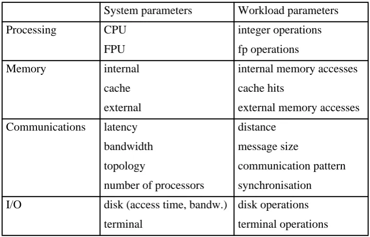
In this paper the second definition is used as the basis for the bottleneck analysis meth-odology which involves the following steps: predict the execution time components of a certain workload, identify the time component responsible for the bottleneck (the slowest part), analyse the component causing the bottleneck into its constituent and identify the sub-components causing the problem. Optimisation of the software subrou-tines and/or hardware utilisation causing the bottleneck can improve the system perfor-mance. This operation can be iterated until no further optimisation is possible. Potential sources of bottlenecks are summarised in Table 1.

Table 1. Sources of potential bottlenecks

In section 2 a background to the bottleneck analysis is given. Section 3 introduces a bot-tleneck analysis methodology based on instruction level analysis. Section 4 provides a case study to illustrate and validate the proposed bottleneck analysis methodology. The case study selected is a communication intensive linear solver algorithm (Gauss-Jordan elimination) which was implemented on a transputer-based mesh connected distributed memory parallel computer (128 T800 Parsytec SuperCluster).

2. Background

A bottleneck in a system is usually the main reason for its performance degradation. A System parameters Workload parameters

Processing CPU integer operations

FPU fp operations

Memory internal internal memory accesses

cache cache hits

external external memory accesses

Communications latency distance

bandwidth message size

topology communication pattern number of processors synchronisation

slow system component affects the performance of the whole system by preventing oth-er components from running at full speed. So it is important to identify these slow com-ponents (software or hardware) and reduce their effects in order to achieve optimal performance.

Gustafson in his paper [Gustafson 91] argues that almost every computer is limited not by the speed of the arithmetic unit but the memory bandwidth and latency. Using sev-eral examples the author showed that this problem is becoming visible even for work-stations not just for parallel computers. Gustafson introduced the idea of characterising the system performance not by the Mflop rate but by the number of delivered Mword/s. Amdahl described the balanced computing system as a system which for each Mflop/s arithmetic performance can deliver 1Mword/s. Amdahl's law states that the perfor-mance enhancement with a given improvement is limited by the amount that the im-proved feature is used [Hennessy 90].

Hollingsworth [Hollingsworth 94] in his thesis describes a monitoring based bottleneck analysis methodology using an iterative process of refining the answers to three ques-tions concerning performance problems. These three quesques-tions are: why is the applica-tion performing poorly, where is the bottleneck, when does the problem occur. The why answer identifies the type of bottleneck (e.g. communication, I/O etc.). The where an-swer isolates a performance bottleneck to a specific resource used by the program (e.g. disk, memory etc.). Answering the when question isolates a specific phase of the pro-gram execution.

Goldberg and Hennessy [Goldberg 90] described a simple monitoring method for de-tecting regions in a program where the memory hierarchy is performing poorly by ob-serving where the actual measured execution time differs from the time predicted given a perfect memory system.

Bottleneck analysis based on instruction code level characterisation has been described by Zemerly [Zemerly 94a]. This approach investigates where the time is spent during the program run. The analysis concentrates on the following components: memory (in-ternal, external), processor (ALU, FPU), communication and I/O.

3. Methodology of Bottleneck Analysis

external), communication (initialisation, distribution, collection etc.) and I/O (disk read/write). These components can be further analysed and potential bottleneck prob-lems can be identified as will be shown later.

3.1. The computation and the memory components

The instruction level characterisation method described in [Zemerly 94b] is used here to predict the performance of the system. The computation component time can be giv-en by:

(1)

For the Parsytec system studied here equation (1) becomes:

(2)

where

t₀ start-up time for vector processors

n_ex total number of cycles to execute the instructions n_mem total number of memory cycles

n_intmem additional time spent to access internal memory n_exmem additional time spent to access external memory

n_inst total number of cycles required to fetch instructions from ex-ternal memory

n_cpu total number of CPU cycles n_fpu total number of FPU cycles

n_{fpu_over} total number of FPU cycles overlapping the CPU t_cyc processor cycle time

3.2. The communication component

Tcomp = τ0 +(νεξ + νµεµ) ×τχψχ

T_comp= (ν_χπυ+ ν_φπυ− ν_{φπυ_ οϖερ}

ν_εξ

1 4 442 4 4 43 + νιντµεµ + ν_νεξτµεµ + νινστ µεµ

The total communication cost can be given by: (3)

where T_init is the initialisation of the communication links (on the Parsytec each link requires 1270 s), T_distis the data distribution time, T_coll is the collection time and T_com is the communication time required in individual stages of the algorithm.

The time of the point-to-point communication depends on the message length (l) and the distance (d) the message has to travel (the number of hops). An analytical commu-nication model for quiet networks is described by Tron [Tron 93]. In this paper a sim-pler communication model based on the work of Bomans [Bomans 89] and Norman [Norman 93] is used and given by:

(4)

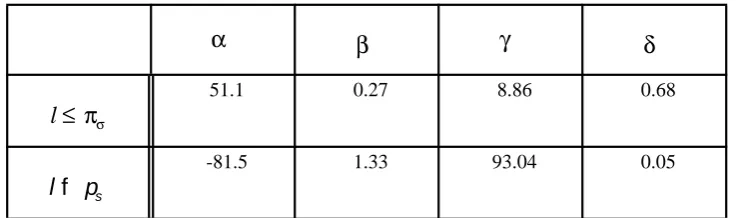
For the Parsytec SuperCluster, the target machine used in this paper, the packet size, ps, is assumed equal to 120 bytes, and the parameters for equation (4) obtained by least square fitting of measured communication times are given in Table 2.

Table 2. Parameters of the quiet network communication model of the Parsytec Super-Cluster

T_dist and T_coll are functions of T_com and will be described later for the case study.

3.3. The I/O component

51.1 0.27 8.86 0.68

-81.5 1.33 93.04 0.05

Ttcom = Τινιτ+ Τδιστ+ Τχολλ+ Τχοµ(λι,δι, πι) ι

σταγεσ

∑

Tcom(l,d)=

α₁+ β₁λ+ γ₁δ + δ₁λδ λ≤ π_σ α₂ + β₂λ+ γ₂δ + δ₂λδ λ> π_σ 

 

α _β γ _δ

l≤ π_σ

The cost of I/O can be analytically expressed by the following formulas (5, 6): (5)

(6)

The coefficients of the formulas above can be obtained by fitting a linear model to mea-surements provided on the target machine. For the Parsytec machine these coefficients are =642.16, =3.73, =1583.73 and =2.2.

3.4. Parallel execution time

The parallel execution time can be derived from the sequential execution time using the non-overlapped computation-communication model for parallel algorithms [Basu 90, Zemerly 94b] and is given by:

(7)

where T_p is the execution time of the algorithm part that can be parallelised. T_s is the execution time of the serial part of the algorithm including initialisation time. T_po is the parallel overhead processing required when parallelising an algorithm, it can only be used when the overhead is known a priori. For example, processing of the data overlap that may be necessary between processors for a domain decomposition problem. T_tcom is the total communication overhead, T_I/Ois the input/output times and U_p is the pro-cessor utilisation and is given by:

Tinput(l)= αρεαδ+βρεαδλ

T_output(l)= α_ωριτε+ β_ωριτελ

α_ρεαδ β_ρεαδ α_ωριτε

β_ωριτε

T_xp(N, p)= Τ_σ+ Τπ

(8)

where p_i is the number of processors active at stage i and T_iis its execution time.

3.5. Bottleneck analysis

A prediction of the components constituting the execution time to identify the slowest part of the system is first carried out using the characterisation method described be-fore. Also three metrics are used to identify bottlenecks in the system, these are the ratio, the communication to computation ratio and memory to processing ratio. The B-ratio (B stands for bottleneck) of an execution time component (i.e. processing, mem-ory, communication and I/O) is the ratio of the component to the sum of all other com-ponents. This metric is dimensionless and a simple comparison between all the B-ratios will clearly identify a bottleneck problem when visualised in the same plot. The best performance is obtained when all the B-ratios are equally balanced and have values less than unity. The communication to computation and memory to processing ratios can be used to identify the communication and memory bottlenecks, i.e. when they exceed uni-ty. These ratios will be used for the bottleneck analysis of the linear solver presented in section 4. Once an execution time component is identified as a bottleneck further anal-ysis of its sub-components can be carried out to highlight any software or hardware re-lated problems causing the bottleneck. This will allow optimisation of software or usage of the hardware resources where possible. These sub-components are: FPU, CPU, external memory, internal memory, initialisation of communication links, data distribution, data collection, other communication overheads, disk read time and disk write time.

4. Bottleneck analysis of large dense systems of linear equations

4.1. Description of the linear solver

In this section the solution of large dense systems of linear equations on a Parsytec

Su-Up= ι πι × Τι

perCluster is described to illustrate the use and validate the bottleneck analysis meth-odology. Linear solvers belong to the computational and communication intensive class of algorithms. A system of linear equations can be represented in the following form:

A X = B (9)

where A is a non-singular square matrix, B is the solution vector and X is a vector of unknowns. There are several solution methods for the system of linear equations which can be classified as direct and iterative methods. In the case of direct methods the amount of computation required can be specified in advance, whereas for the iterative methods the number of computation steps depends on the value of the initial solution vector and the required precision. Typical examples of the direct methods are Gauss elimination with back substitution, Gauss-Jordan elimination, LU, QR and Cholesky factorisations [Barnett 90, Modi 88]. The iterative methods are based on Jacobi or Gauss-Seidel algorithms [Champion 93].

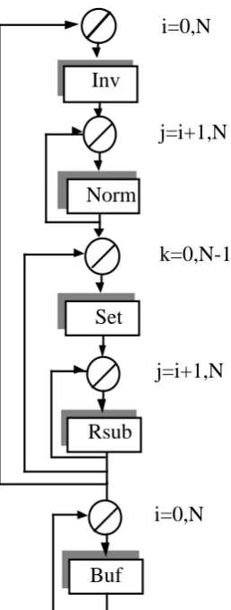
Figure 1. Software execution graph for the sequential linear solver

The computational blocks shown in Figure 1 are:Inv- calculate the inverse of the pivot element, Norm- normalisation of the actual row, Set- variable setting, R row sub-traction and Buf- data buffering.

The sequential execution time for the linear solver can be given by: (10)

where t_i is the number of cycles for module i.

4. 2. Parallel linear solver

The diagonalisation of the initial matrix requires N algorithmic steps (k =1,N) and each step consists of the sequence of the following operations: normalisation of the k-th row,

i=0,N

j=i+1,N

k=0,N-1

j=i+1,N Set

Norm Inv

Rsub

Buf

i=0,N

T_x(N)= τ_Ινϖ+ τ_Νορµ+ τ_Σετ+ τ_Ρσυβ ϕ=ι+1

Ν

∑

κ=0 Ν−1

∑

ϕ=ι+1 Ν

∑

 

 

 

ι= 0 Ν

∑

ι=1 Ν

broadcasting the k-th row to all the processors and updating the submatrix on all the processors.

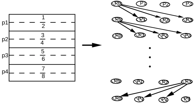
The parallel linear solver can be obtained by extending the sequential algorithm with communication routines which provide distribution of input data, broadcasting and col-lection of output data during the algorithm execution. The block-row data decomposi-tion which divides the matrix horizontally and assigns adjacent blocks of rows to neighbouring processors is considered here. The matrix decomposition and the commu-nication graph for four processors are presented in Figure 2.

Figure 2. Block row data decomposition and the communication graph

Assuming that T_sand T_po are negligible and U_p is 1 in equation (7), the parallel execu-tion time for the linear solver can be given by:

(11) where (12) (13) 1 2 3 4 5 6 7 8 p1 p2 p3 p4

P1 P2 P3

P0 _P2 P3

P1 P2 P3

P1 _P2 P3

P0 P1 P2 P3

P0 P0 P1 P0 • • •

T_xp(N, p)= Τξ(Ν)

π + Τδιστ+ Ν × Τβροαδ+ Τχολλ+ ΤΙ/ Ο

Tdist = Τχοµ ι=1

π

∑

Tcoll = Τχοµ(λι ι=1

π

(14)

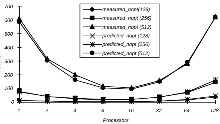
The value of l_i for distribution is (N/p)*(N+1)*8, for collection is (N/p)*8 and for broad-casting is (N+1)*8. The parameter d_i,j is the distance between processors i and j. The linear solver algorithm was implemented on the Parsytec machine and the execution times were measured to validate the predictions. The results of the predictions and the measurements for various task sizes (128, 256 and 512 equations) and number of pro-cessors are given in Figure 3 and Table 3.

Figure 3. Predictions and measurements for the non-optimised linear solver

Table 3. Predictions and measurements for non-optimised linear solver

1 2 4 8 16 32 64 128

measured_nopt(128) 10.13 5.65 4.05 3.4 4.47 8.73 17.33 36.56

measured_nopt (256) 78.21 41.52 27.21 18.91 20.91 36.03 69.81 146.27

measured_nopt (512) 612.35 317.93 198.06 116.48 104.07 156.49 283.32 622.91

predicted_nopt (128) 9.51 5.48 3.5 3.24 4.49 9.11 19.53 44.89

predicted_nopt (256) 74.26 39.98 23 17.32 19.75 36.12 73.41 160.9

predicted_nopt (512) 586.52 304.78 164.32 105.24 96.4 151.62 291.77 624.61 T_broad = Τ_χοµ(λ_ι

ι=0 π

∑

Processors

Time, s

0 100 200 300 400 500 600 700

1 2 4 8 16 32 64 128

measured_nopt(128)

measured_nopt (256)

measured_nopt (512)

predicted_nopt (128)

predicted_nopt (256)

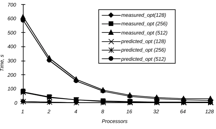
Note that the broadcast used here is based on a simple one-to-all communication. A de-tailed analysis of the results identified a bottleneck in the communication component which is represented by the broadcast subroutine. This subroutine was then optimised using neighbourhood communication. A sample of the bottleneck analysis which was carried out on the non-optimised code will be given for the final version of the code in-stead. Figure 4 and Table 4 show the execution time measurements and predictions for the optimised linear solver.

Figure 4. Execution time prediction and measurements of the optimised linear solver

Table 4. Predictions and measurements for the optimised linear solver

The broadcast time used here can be given by:

1 2 4 8 16 32 64 128

measured_opt(128) 10.13 5.63 3.36 2.31 1.82 1.72 1.85 2.34

measured_opt (256) 78.15 41.33 22.67 13.73 9.4 7.46 6.89 7.54

measured_opt (512) 612.26 316.85 166.41 92.35 55.21 38.22 30.5 29.3

predicted_opt (128) 9.51 5.35 3.03 1.9 1.4 1.26 1.47 2.16

predicted_opt (256) 74.26 39.48 21.12 12 7.55 5.52 4.99 5.62

predicted_opt (512) 586.52 302.79 156.83 83.99 47.79 30.06 22.13 19.69

Processors

Time, s

0 100 200 300 400 500 600 700

1 2 4 8 16 32 64 128

measured_opt(128)

measured_opt (256)

measured_opt (512)

predicted_opt (128)

predicted_opt (256)

(15)

As can be seen from the results above the introduction of optimised broadcast subrou-tine provided good scalability for the algorithm.

4.3. Results of the bottleneck analysis for the optimised code

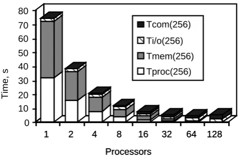
The results in Figures 5, 6 show the components of the execution time: processing, memory, communication and I/O for 256 linear equations for various number of pro-cessors.

Figure 5. Processing, memory, communication and I/O times Tbroad = Τχοµ(λι

νειγηβουρσ

∑

,1)

1 2 4 8 16 32 64 128

Processors 0

10 20 30 40 50 60 70 80

Time, s

1 2 4 8 16 32 64 128

Processors

Tcom(256)

Ti/o(256)

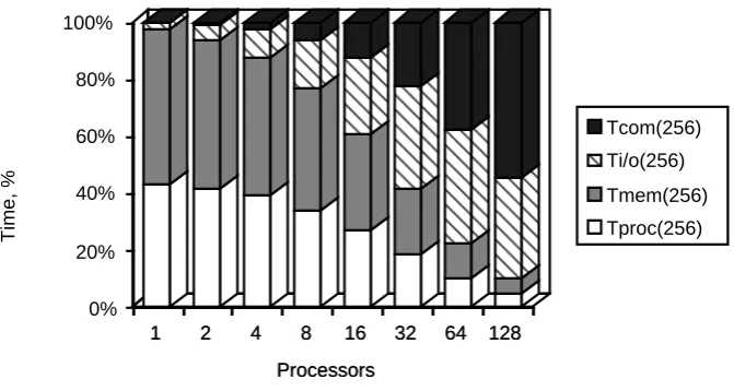
Figure 6. Processing, memory, communication and I/O percentages

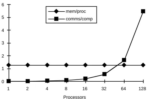
Figures 7 and 8 show the B-ratio and the communication-computation ratio for 256 equations for various numbers of processors.

Figure 7. B-ratio for processing, memory, communication and I/O for 256 equations

1 2 4 8 16 32 64 128

Processors 0%

20% 40% 60% 80% 100%

Time, %

1 2 4 8 16 32 64 128

Processors

Tcom(256) Ti/o(256)

Tmem(256)

Tproc(256)

Processors

B-ratio

0 0.2 0.4 0.6 0.8 1 1.2

1 2 4 8 16 32 64 128

Bproc Bmem

Bcomm

Figure 8. Communication-computation and memory-processing ratios for 256 equa-tions

As can be seen from Figure 7 the communication becomes a bottleneck after 64 proces-sors while the I/O time is a bottleneck between 16 and 64 procesproces-sors. Figure 8 shows that the communication-computation ratio exceeds unity at around 48 processors and hence the communication is becoming a potential bottleneck after that number. The memory-processing ratio is constant throughout because of the absence of a cache memory level on the Parsytec system. This ratio will show clearly the effect of cache in systems where it exists. Figure 9 and Table 5 show the breakdown of execution time components for various number of processors for 256 equations.

Processors 0

1 2 3 4 5 6

1 2 4 8 16 32 64 128

mem/proc

comms/comp

1 2 4 8 16 32 64 128

Processors 0%

20% 40% 60% 80% 100%

Time, %

1 2 4 8 16 32 64 128

Processors

Tcoll(256) Tbroad(256)

Tdist(256)

Tcini(256) Tout(256)

Tinp(256)

Tinmem(256) Texmem(256)

Tcpu(256)

Figure 9. Breakdown of execution time components

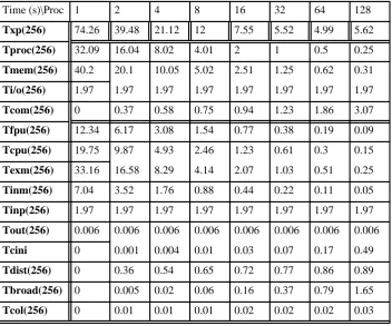
Table 5. Breakdown of execution time components

Figure 9 shows clearly that T_inp becomes a major bottleneck starting from 32 processors and for 128 processors T_broad becomes another potential bottleneck.

5. Conclusions

A bottleneck analysis methodology for parallel systems based on characterisation has been described. A characterisation method used here is based on the instruction level analysis used in [Zemerly 94b]. A case study on a communication intensive algorithm has been presented to illustrate and validate the bottleneck analysis methodology. The execution time measurements obtained from running a parallelised version of the linear solver on the target machine were compared with the predictions and showed an aver-age error of about 15%. Three bottleneck metrics were successfully used in the analysis to identify the execution time components causing the bottlenecks. The analysis iden-tified a bottleneck problem in the algorithm and a part of the code causing the bottle-neck was optimised resulting in a significant performance improvement.

Time (s)\Proc 1 2 4 8 16 32 64 128

Txp(256) 74.26 39.48 21.12 12 7.55 5.52 4.99 5.62

Tproc(256) 32.09 16.04 8.02 4.01 2 1 0.5 0.25

Tmem(256) 40.2 20.1 10.05 5.02 2.51 1.25 0.62 0.31

Ti/o(256) 1.97 1.97 1.97 1.97 1.97 1.97 1.97 1.97

Tcom(256) 0 0.37 0.58 0.75 0.94 1.23 1.86 3.07

Tfpu(256) 12.34 6.17 3.08 1.54 0.77 0.38 0.19 0.09

Tcpu(256) 19.75 9.87 4.93 2.46 1.23 0.61 0.3 0.15

Texm(256) 33.16 16.58 8.29 4.14 2.07 1.03 0.51 0.25

Tinm(256) 7.04 3.52 1.76 0.88 0.44 0.22 0.11 0.05

Tinp(256) 1.97 1.97 1.97 1.97 1.97 1.97 1.97 1.97

Tout(256) 0.006 0.006 0.006 0.006 0.006 0.006 0.006 0.006

Tcini 0 0.001 0.004 0.01 0.03 0.07 0.17 0.49

Tdist(256) 0 0.36 0.54 0.65 0.72 0.77 0.86 0.89

Tbroad(256) 0 0.005 0.02 0.06 0.16 0.37 0.79 1.65

Bibliography

Barnett 90 S. Barnett. Matrices Methods and Applications, Clarendon Press, Oxford 1990.

Basu 90 A. Basu, S. Srinivas, K. G. Kumar, A. Paulraj. A Model for Performance Pre-diction of Message Passing Multiprocessors Achieving Concurrency by Do-main Decomposition. Proc. of the Joint Int. Conf. on Vector and Parallel Processing, (editor) Burkhart, H., Lecture Notes in Computer Science, 457, 10-13 September, Zurich, Switzerland, Springer-Verlag, pp. 75--85, 1990.

Bomans 89 I. Bomans and D. Roose. Benchmarking the iPSC/2 Hypercube Multicom-puter. Concurrency: Practice and Experience 1 (1), pp 3-18, 1989.

Champion 93 E. R. Champion. Numerical Methods for Engineering Applications. Marcel Dekker, Inc, 1993.

Goldberg 90 A. Goldberg, J. Hennessy. MTOOL. A Method for Detecting Memory Bot-tlenecks. WRL Technical Note TN-17, Palo Alto, California, 1990.

Gustafson 91 J.L. Gustafson. Computer Intensive Applications on Advanced Computer Applications, D .J. Evans, G. R. Jouber and H. Lidell (Editors), Parallel Com-puting, pp. 75-89, 1991.

Hennessy 90 J. L. Hennessy and D. A. Patterson. Computer Architecture: A Quantitative Approach, Morgan Kaufmann Publishers, 1990.

Hollingsworth 94 J. K. Hollingsworth. Finding Bottlenecks in Large Scale Parallel Programs. PhD Thesis, Dept. of Computer Science, University of Wisconsin-Madison, 1994.

Modi 88 J. J. Modi. Parallel Algorithms and Matrix Computation, Clarendon press, Oxford, 1988.

Norman 93 M. G. Norman and P. Thanish. Models of Machines and Computation for Mapping in Multicomputers. ACM Computing Surveys, vol 25, no.3, Sep-tember, pp 263-301, 1993.

Smith90 C. U. Smith. Performance Engineering of Software Systems . Addison-Wes-ley Publishing Co. Inc., 1990.

Tron 93C. Tron and B. Plateau. Modelling Communication in Parallel Machines Proc.Performance

Evaluation of Parallel Systems, University of Warwick, UK, pp 110-117,

De-cember 1993.

Zemerly 94a M. J. Zemerly, G. R. Nudd, T. J. Atherton, D. J. Kerbyson, E. Papaefstathiou, J. Papay and R. Ziani. Analysis of Bottlenecks. ESPRIT III PEPS Project (6942) Interim Report, University of Warwick, January 1994.