ACCELERATED MORPHOLOGICAL MODELLING
A SCHEMATIZED CASE STUDY INTO THE MEDIUM- AND LONG-TERM
MORPHOLOGICAL ACCELERATION TECHNIQUES MORFAC AND MORMERGE
ARCADIS & UNIVERSITY OF TWENTE
M.Sc. Thesis R.J.A. Wilmink
ACCELERATED MORPHOLOGICAL MODELLING
A schematized case study into the medium- and long term morphological acceleration
techniques Morfac and Mormerge
Thesis
Submitted to acquire the degree of Master of Science To be presented in public
On 7 July 2015 at 15.00 hours
At University of Twente, Enschede, the Netherlands
By
Rinse Johannes Andreas Wilmink
University of Twente
Faculty of Engineering Technology
Master Programme: Civil Engineering and Management, Water Engineering and Management Student number: s1095153
This thesis has been approved by the supervisors.
Members of graduation committee:
Dr. ir. J.S. Ribberink Chairman, University of Twente
Water Engineering and Management, Marine and fluvial systems Dr.ir. P.C. Roos Supervisor, University of Twente
Water Engineering and Management, Marine and fluvial systems Dr. A.P. Tuijnder Supervisor, Arcadis, River, Coast and Sea & University of Twente Dr. ir. B.T. Grasmeijer Supervisor, Arcadis, River, Coast and Sea
Abstract
In simulating the long-term morphology of a natural coastal and offshore system, the most restrictive element is the available computational capacity. Computations for long-term simulations of the morphology take a long time and a lot of computational power. To overcome this crucial disadvantage for long-term morphological simulations, input reduction for real-time measurement signals and an acceleration of morphological changes can be applied. This thesis attempts to test both approaches. Based on progressive insight in morphodynamic modelling, two techniques for accelerating the morphological changes are commonly used nowadays, i.e. Morfac and Mormerge. The performance of both methods and their possibilities and limitations for a uniform sandy coast, including a navigation channel and a harbour entrance is the subject of this study.
This thesis first provides answers to introductory questions as which input conditions should be combined into ‘input scenarios’ to run morphological simulations that represent the reality and how do Morfac and Mormerge simulate the medium- and long-term morphology. Then, using a schematized Delft3D model in 2DH mode for the coastal and offshore area of IJmuiden, there has been investigated in what way a tidal signal can be reduced, how many wave classes should be included to obtain accurate results, which acceleration factor is still acceptable to achieve accurate results and what are the distinguishing elements that decide which method is most appropriate for a certain simulation. All simulations will produce a ten yearly morphodynamic development of the study area by tidal forcing (and if included, waves as well). The simulations are compared to a reference simulation. To quantify the accuracy, four performance indicators will be calculated. These performance indicators are: Nash-Sutcliffe coefficient (NS), Root Mean Square error (RMS), linear correlation coefficient (R) and the slope of the linear regression line (B). An acceptable accurate result is obtained when the NS is above 0.95, the RMS lower than 0.5, R over 0.99 and B lower than 1.05. By means of a Multi-Criteria-Analysis (MCA) a comparison will be performed between Morfac and Mormerge. The assessment criteria of the MCA are: accuracy, ease of use, applicability (physical justification of what is happening) and simulation time.
The reference simulation chosen in this study is named the brute-force simulation. This brute-force simulation uses the reduced tidal input condition, a measured wave signal and an acceleration factor of ten to simulate the morphological development for ten years. Incorporating these elements for the brute-force simulation is the most time efficient and closest to reality as possible for the time limit of this study.
Morfac and Mormerge both accelerate the sediment transport rate by a factor. This approach is considered legitimate because of the differences in timescales of the hydro- and morphodynamics. The difference between the techniques is in the computation of particular conditions (for example varying wave heights or directions). Morfac calculates the conditions one after another using the bathymetry of the previous condition at the start of the new condition. The acceleration factor applied is for every condition multiplied by a weight (percentage of occurrence of that particular condition). The sequence of conditions is determined randomly. Mormerge calculates these conditions parallel by weighting the bottom change of all conditions every flow time step by its percentage of occurrence of that condition. A fixed acceleration factor is applied in Mormerge.
harmonic to avoid shocks of the model from one tide to another and it consists of the M2, M4, M6 and M8
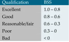
tidal constituents. For the long-term simulations, the harmonic morphological tide is easy to implement. The validation of the harmonic morphological tide, when focusing on water levels and flow velocities, matches the double tide of the spring-neap tidal cycle very well. The Nash-Sutcliffe coefficients averaged over 41 temporal observation points in the domain for the water levels and flow velocities are 0.98 and 0.95 respectively. The Brier Skill Score of the morphological development by the harmonic morphological tide compared to the morphological development of the simulated spring-neap tidal cycle is 0.96 (were a value of 1 is a perfect prediction with respect to the brute-force simulation). In addition, a real-time wave signal has been converted into directional and magnitudinal bins. The results of short simulations of all combinations of directional and magnitudinal bins (wave conditions) have been used to determine the sequence of importance for the morphological development of the study area by different wave conditions. This sequence is determined by the OPTI-routine which resulted in four wave scenarios (including one, two, six or ten wave classes).
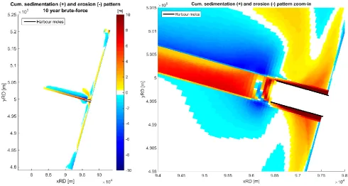
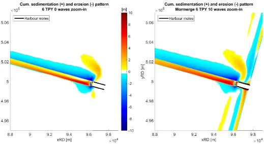
The long-term simulations performed showed the formation of nearshore banks, migration of the nautical channel, sedimentation around the harbour moles and a deep scour hole directly in front of the harbour moles. This study showed that for water depths of approximately > 6 m, the acceleration factor and acceleration method are not decisive for the accuracy of the results with respect to the brute-force simulation (in water depths over 6 m, the sediment transport is more tide driven). The model is accelerated to its maximum factor possible using the input reduction for the tide; at least one harmonic morphological tide has to be simulated for the result to be valid. No deviating results were obtained. The inclusion of additional wave classes (determined by the OPTI-routine) resulted in an increased model performance. At least six wave classes had to be included to obtain results within the acceptable range of accuracy.
Samenvatting
De beschikbare rekenkracht van computers is tegenwoordig nog steeds de meest beperkte factor bij het simuleren van natuurlijke kust en zee systemen. Morfodynamische simulaties voor de langere termijn zijn tijdrovend en kosten veel rekenkracht. Om deze nadelige bijkomstigheid in te dammen kan een input reductie van meetsignalen in de tijd dan wel een versnelling van de morfologische veranderingen worden toegepast. Deze studie is een combinatie van beide opties. Voor de versnelling van de morfologische veranderingen zijn Morfac en Mormerge hedendaags het meest gebruikt. Deze methoden zijn gebaseerd op voortschrijdend inzicht in morfodynamisch modelleren. De prestatie van beide methoden en de voor- en nadelen voor een zandige kust met een vaargeul en haveningang, zijn het onderwerp van deze thesis.
Dit onderzoek zal allereerst twee introducerende vragen beantwoorden: welke input condities moeten combineert worden tot input scenario’s om morfologische simulaties vergelijkbaar met de werkelijkheid te kunnen uitvoeren en hoe simuleren Morfac en Mormerge de langere termijn morfologie? Vervolgens, gebruik makende van een geschematiseerd Delft3D model in 2DH mode voor het kust- en offshore gebied van IJmuiden, is onderzocht hoe het getijsignaal kan worden gereduceerd, hoeveel golfklassen moeten worden meegenomen voor goede simulatieresultaten, welke acceleratiefactor is nog acceptabel om goede resultaten te behalen en wat de onderscheidende elementen zijn die bepalen welke methode het best gebruikt kan worden voor een bepaalde situatie? Alle simulaties zullen een tienjarige morfodynamische verwachting van het studiegebied simuleren door gebruik te maken van getij (en wanneer meegenomen, golven). De simulaties worden vergelijken met een referentiesituatie. Om de nauwkeurigheid van de simulaties te kwantificeren worden vier criteria berekend. Deze criteria zijn de Nash-Sutcliffe coëfficiënt (NS), Root Mean Square error (RMS), lineaire correlatiecoëfficiënt (R) en de helling van de lineaire regressielijn (B). Het nauwkeurigheidsniveau vereist voor een acceptabele simulatie wordt bereikt wanneer de NS coëfficiënt boven 0.95 is, de RMS lager dan 0.5, R hoger dan 0.99 en B lager dan 1.05. Een Multi-Criteria Analyse (MCA) vergelijkt de verschillen tussen de versnellingsmethoden, meegenomen golfklassen en versnellingsfactoren. De beoordelingscriteria van de MCA zijn: nauwkeurigheid, gebruiksgemak, toepasbaarheid (fysische verklaarbaarheid van wat er gebeurt) en rekentijd.
De referentiesituatie van deze studie wordt de brute-force simulatie genoemd. Deze brute-force simulatie maakt gebruikt van het reduceerde getijsignaal, een gemeten golfsignaal en een versnellingsfactor van tien om een tienjarige morfologische ontwikkeling te simuleren. Het gebruik van deze elementen in de brute-force simulatie is het meest tijd efficiënt en ligt het dichtst bij de realiteit voor de tijdslimiet van de studie.
Voor de inputreductie van het model is een morfologisch getij afgeleid welke de morfologische verandering van een volledige springtij-doodtij cyclus zo nauwkeurig mogelijk nabootst. Deze nauwkeurigheid is gemeten door middel van de lineaire correlatiecoëfficiënt. Om schokken in het model te voorkomen (van het ene naar het andere getij) is het morfologisch getij harmonisch gemaakt. Dit harmonische morfologische getij bestaat uit vier getijdecomponenten te weten M2, M4, M6 en M8. Dit
gereduceerde harmonische getij is eenvoudig te implementeren voor de lange termijn simulaties. In de validatie van het harmonische morfologische getij, vergeleken met waterstanden en stroomsnelheden, presteert dit getij erg goed vergeleken het getij van de springtij-doodtij cyclus. De Nash-Sutcliffe coëfficiënt gemiddeld over 41 observatiepunten in het domein van de waterstanden en de stroomsnelheden zijn 0.98 en 0.95 respectievelijk. De Brier Skill Score van de morfologische ontwikkeling veroorzaakt door het harmonische morfologische getij vergeleken met de morfologische ontwikkeling van de gesimuleerde springtij-doodtij cyclus is 0.96 (hierbij geeft een waarde van 1 een perfecte voorspelde ontwikkeling ten opzichte van een referentiesituatie aan). Voor de input reductie van de golven is het gemeten golvensignaal onderverdeeld in hoogte- en richtingsklassen. Voor elke combinatie van een hoogte- en richtingsklasse is een korte morfologische simulatie uitgevoerd. De resultaten van deze simulatie zijn gebruikt om de volgorde te bepalen van de mate waarin een specifieke conditie (combinatie van golfhoogte en richting) de totale morfologische ontwikkeling van het gemeten signaal nabootst. Deze volgorde is bepaald door de OPTI-routine methode en heeft geleidt tot vier verschillende golfklimaten (de golfklimaten bestaan uit één, twee, zes of tien golfklassen).
Alle uitgevoerde lange termijn simulaties laten duidelijk de formatie van kustnabije zandbanken, de migratie van de vaargeul, de ontwikkeling van de erosiekuilen en de sedimentatie direct voor de havendammen zien. In deze studie komt naar voren dat voor waterdieptes ongeveer groter dan 6 m de acceleratiefactor en methode niet bepalend zijn voor de nauwkeurigheid van het resultaat (t.o.v. de brute-force simulatie). In waterdiepten groter dan 6 meter is het sedimenttransportsysteem meer getij gedreven dan golf gedreven. Het model is hierbij versneld tot het maximum mogelijk wanneer men gebruikt maakt van deze inputreductie voor het getij; tenminste 1 harmonisch morfologisch getij moet gesimuleerd worden voor een valide resultaat. Geen significante verschillen in de resultaten konden worden geobserveerd. Het meenemen van extra golfklassen (bepaald door de OPTI-routine) resulteert wel in een verbeterde model prestatie. Tenminste zes golfklassen moeten worden meegenomen in de simulatie om een voldoende nauwkeurigheidsniveau te bereiken.
Preface
Five years ago, on the 30th of August 2010, my first lecture in Civil Engineering took place. The more I got
into the field of Civil Engineering; it became clear that water is my subject. Choosing the track Water Engineering and Management, flooding, flood protection, flood risks, drought, water policy and standards, propagation of water and sediment, measurements and data analysis, physics, design and engineering, all subjects passed by. During the master phase, it also became clear that the understanding of water (and sediment/morphology) is still limited. Testing of hypotheses’ and thoughts of how the natural system works costs a lot of effort. Increased computational capacities have eased this work. However, making a prediction of a very long time span for a system where the conditions are changing from second to second is still very difficult and very much restricted by the computational capacity available. I hope that this master thesis contributes to the knowledge, especially in engineering practice, about how and how fast the long term predictions for a morphodynamic system can be accelerated and what the advantages and disadvantages are. Understanding of the natural forces acting on the system to be simulated is essential to evaluate the results of the simulations.
Writing this thesis, a period of five years being a student is almost completed. These five years flew by very fast. Being a student offered a lot of opportunities to visit many projects in my field of interest. In addition, it offered several opportunities to visit places far away and experience different cultures. I would like to thank many people who made these five years very nice and pleasant (In Dutch there is a word for this: ‘’Gezellig’’. However, no English translation exists that exactly means the same…..).
First of all, I would like to thank my family for the support and patience in the past five years. I would like to thank my friends for always being interested in my work, for the nice activities, nights out and for the trips we made. Hopefully many more will come. Besides, I would also like to thank my colleagues at ARCADIS River, Coast and Sea. They supported me, helped me out when I got stuck and inspired me for this research. Especially, Arjan Tuijnder for his supervision and providing feedback and Bart Grasmeijer for helping me out with the model, enthusiastic discussions about the topic, answering my always very simple questions and bringing me coffee!
At the university I would like to thank Jan Ribberink for his critical reviews and discussions of my work. A special thank goes to Pieter Roos. Using his network I got the opportunity to perform this master thesis at ARCADIS. He supervised this master thesis and provided very detailed feedback. With this feedback (also from Arjan, Bart & Jan) I was able to improve this thesis. Besides, Pieter, also thanks for being constructive and to think along with us to make it possible to follow a course when we were in South-America!
Rinse
Contents
Abstract ... III
Samenvatting ... V
Preface ... VII
1 Introduction ... 3
1.1 Research background ... 3
1.2 Problem description & Objective ... 4
1.2.1 Research objective ... 4
1.2.2 Research questions... 5
1.3 Methodology and reading guide ... 5
2 Study area ... 9
2.1 Introduction ... 9
2.2 Study area ... 9
2.3 Characteristics of tide and waves ... 10
2.3.1 Tide ... 10
2.3.2 Waves ... 11
3 Morphological acceleration techniques in numerical modelling... 13
3.1 Introduction ... 13
3.2 Morfac ... 14
3.3 Mormerge ... 16
3.4 Similarities and differences of Morfac and Mormerge ... 16
4 Model setup ... 18
4.1 Delft3D process-based model ... 18
4.2 Grid ... 18
4.3 Numerical parameters... 19
4.3.1 Initial Bathymetry ... 19
4.3.2 Boundary conditions ... 21
4.3.3 Other Parameters and settings ... 22
4.3.4 Initial conditions ... 22
5 Input reduction ... 23
5.1 Tide schematization ... 23
5.2 Wave Schematization ... 26
5.3 Validation of input reduction ... 29
5.3.1 Framework ... 29
5.3.2 Results ... 31
5.4 Summary input reduction ... 32
6 Results long-term morphological modelling ... 33
6.1 Validation Brute-Force simulation ... 33
6.3 Comparison of performance parameters long-term simulations ... 42
6.4 Summary ... 44
7 Multi-Criteria Analysis ... 45
7.1 Framework ... 45
7.2 Results of the Multi-Criteria Analysis ... 46
8 Discussion and Conclusions ... 47
8.1 Discussion ... 47
8.1.1 Input Reduction ... 47
8.1.2 Long-term accelerated simulations ... 48
8.2 Conclusions ... 49
8.3 Recommendations ... 51
Bibliography ... 52
List of Figures ... 55
List of Tables ... 58
Appendices ... 59
A. Delft3D model description ... 59
A.1. Hydrodynamics ... 59
A.2. Sediment transport and Morphology ... 60
A.3. Wave Module ... 61
A.4. Grid & Boundary conditions ... 61
A.5. Solution procedure ... 62
A.6. Numerical parameters Delft3D model... 62
B. Input reduction ... 65
B.1. Correlation and spreading of all combinations of double tides ... 65
B.2. Sand transport after spring-neap tidal cycle... 66
B.3. Combinations of realistic and occurred wave heights and directions ... 66
B.4. Defined wave climates based on OPTI-method ... 68
B.5. Validation results ... 69
C. Long-term Morphological Modelling ... 70
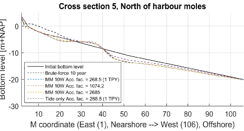
C.1. Cross section results for different acceleration factors ... 70
C.2. Cross section results for inclusion of different wave classes ... 78
1
Introduction
1.1
RESEARCH BACKGROUNDEvery day, many ships are entering and leaving the harbour of Rotterdam through the Euro-Maasgeul for all kinds of purposes. Ships with a maximum draft of 22.85 m are allowed to use the Euro-Maasgeul in the North Sea (Rijkswaterstaat, 2014). Behind the breakwaters of this waterway, at the coast, sandy beaches and dunes are present which protect the hinterland from flooding. Besides, they are of great touristic and economic value. The presence of this beach next to the nautical waterway means that the waterway incises the up-sloping sea bottom towards the coast.
Other examples in which the development of the (coastal) morphology to human activities is relevant are: cables and pipelines, offshore windfarms, oil platforms and other hydraulic structures, all founded on the bottom of a waterbody. These structures, including the nautical channels, are often present for several decades and are of great value for the world economy (e.g. internet cables). Because of the presence of highly economically valued items on the bottom of the sea, it is important to have a clear understanding of their complex behaviour. Morphodynamic models for the medium- and long-term are indispensable tools to understand this behaviour and to predict what will happen in the future.
The behaviour of the hydrodynamics and morphodynamics is affected by each other (Ranasinghe et al., 2010; Ribberink, 2011; Wijnberg, 1995). The hydrodynamics are changing the layout of the bottom through sediment transport and, in turn, the bottom layout changes the behaviour of the hydrodynamics, be it on different timescales. Modelling this mutual behaviour is difficult because of the interactive character of the hydro- and morphodynamics. In addition, the input conditions used for these models are changing in time, even from second to second. One can think of a varying wind speed and direction resulting in waves and currents that in turn interact with the tide and the morphology, thus changing the water levels and sediment transport. Also, not every grain on the sea bottom can be described individually with its particular shape and size. When all relevant physical processes would be included in a numerical model that simulates a couple of years of morphological changes, long run times of the simulation are needed because of the enormous number of calculations that have to be executed using the restricted computational capacity. Therefore, morphological modelling, especially in the vicinity of a coast, needs a form of process aggregation or information reduction (De Vriend, et al., 1993; Lesser, 2009).
According to De Vriend et al. (1993) three distinct approaches for medium- and long-term morphological modelling can be used:
Input reduction. This is based on the idea that residual long-term effects can be described with models based on the description of small-scale processes forced with reduced representative inputs.
Behaviour-oriented modelling. This approach only models the phenomenon of interest without understanding and describing the underlying processes.
This thesis employs a combination of the first two approaches: input reduction and model reduction to simulate the long-term morphological behaviour. Besides the input aggregation and a schematization of reality, often an acceleration of the morphological development is applied to reduce the computational effort and to obtain the results more quickly. For this model reduction, the acceleration factors (multipliers) are applied to the suspended and/or bed load sediment transport rates.
Amongst others, some very often and widely applied morphological medium- and long-term acceleration methods, for example applicable in Delft3D, are: Tide-averaging, Continuity-correction, Rapid Assessment of Morphology (RAM), Morfac and Mormerge (Roelvink & Reniers, 2012). These methods have been developed on the basis of progressive insight in morphodynamic modelling and the most efficient use of the available computational power. The most common and currently used methods to accelerate morphodynamic simulations are Morfac and Mormerge. These methods are more extensively described in section 3 of this thesis. Both methods include an acceleration factor for the morphological changes and are the subject of this thesis.
Several studies have shown good applicability of Morfac and Mormerge for modelling the medium- and long-term morphodynamics, e.g. Lesser et al. (2004); Lesser (2009); Van der Wegen & Roelvink (2008); Zimmerman et al. (2012). They can be implemented in various numerical models as Delft3D (Deltares), Mike21 (Danish Hydraulic Institute) and Telemac (Laboratoire Nationale d’Hydraulique, France). Example implementations of one of the morphological acceleration techniques in Delft3D, Mike 21 and Telemac can be found in the studies of Lesser et al. (2004), Jimenez & Mayerle (2010) and Knaapen & Joustra (2012) respectively. For this study, the numerical model Delft3D will be used (Open Source version 4168, in 2DH mode as will be explained in section 2).
1.2
PROBLEM DESCRIPTION & OBJECTIVEIn engineering practice several methods, as mentioned above, are nowadays used, e.g. in Delft3D, to simulate the medium- and long-term morphological behaviour of water bodies. The most common, recent and computationally efficient methods used are the Morfac and Mormerge. The focus in this thesis is on these two methods which are developed based on progressive insight in accelerated morphological modelling. The working procedures of these methods are explained in section 3.
Which of the two methods performs best under particular circumstances compared to a reference simulation (or reality), however, is not known. In practice several assumptions are made how to include the many different input conditions, their interaction and which morphological acceleration factor is still acceptable for a reasonable simulation. The choice as to which method will yield the best results is merely based on experience of the researcher and is the problem definition of this thesis.
1.2.1
RESEARCH OBJECTIVEtime and the applicability for a particular situation are important criteria for assessing the results of a certain method.
For this study, the emphasis is not on the calibration and validation of a morphological model for the study area. No specific attention will be paid to the influence of numerical parameters. The model built in this study will be used to address the influence of input reduction and of different acceleration methods compared with each other and to the situation without morphological acceleration and input reduction.
1.2.2
RESEARCH QUESTIONSTo achieve the above objective, several research questions are defined:
1. Which input conditions should be combined into ‘input scenarios’ to run morphological simulations that represent the reality?
2. How do Morfac and Mormerge simulate medium- and long term morphology? a. Which model equations are solved during the simulation and in what sequence? b. Which extra options are available in the execution?
c. Which feedback loops between the morphodynamics and hydrodynamics are present and what are they doing?
d. Are there any significant differences in the working procedures of the two methods resulting in significantly different results?
3. In what way can a real-time tidal signal be reduced to a representative tide that is able to simulate accurate hydrodynamic and morphodynamic results compared to a reference period?
4. How many wave classes resulting from the input reduction should be included in a simulation using Morfac and Mormerge to obtain accurate results compared to a reference simulation? 5. Which acceleration factor for the morphological changes is still acceptable to achieve accurate
results compared to a reference simulation?
6. What are the distinguishing elements that decide which method is most appropriate for a certain simulation?
1.3
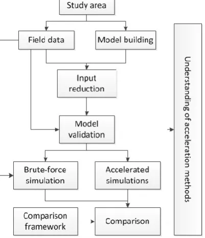
METHODOLOGY AND READING GUIDEDuring this research, several steps based on the research questions will be performed to achieve the objective of this thesis. An overview of these steps is given in Figure 1. First, the study area for which a schematized model will be constructed is described (section 2). This description includes field data characteristics and reveals important hydrodynamic elements of the natural system. These elements should be included in the simulations to represent reality and will provide an answer for research question one.
A schematisation of the study area is chosen for simplicity. The schematized model should represent an existing situation for the practical application of the results. The study site chosen consists of the coastal and offshore area of IJmuiden, the Netherlands. Because of the relatively low fresh water discharge due to sluices and locks located at the canal entrance near the sea, on average only 95 m3/s (Swinkels, Bijlsma, &
version 4168). For this model, a so-called online approach in Delft3D is used. The online approach differs from an offline approach where the wave module uses the outcomes of the flow computations. In the online approach, the wave field in the flow module is updated periodicaly based on the most recent flow field results. The flow module in turn uses the most recently calculated wave field to compute a new flow field and sediment transport field (Deltares, 2014).
Figure 1 - Research approach visualised
To answer research question two, a thorough understanding of the morphological acceleration methods of interest is needed. In section 3, a detailed description of Morfac and Mormerge, and how these methods simulate the long-term morphology, is provided. This description includes information about the implementation of the acceleration methods in this study. In section 4, the schematized model will be set-up including grid building, bathymetry construction and definition of the boundary segments for the boundary conditions.
In section 5 the input reduction will be performed. Because of the continuously changing conditions of the system, a form of process aggregation is needed to avoid long run times of the simulations. The input reduction will be applied for the tide and the waves. These aggregated processes of tide and waves form the base of the long-term simulations. Several different scenarios will be built from simple (tide only) to more complex (tide – wave interactions and different wave heights/directions) which serve as input for the long-term simulations1. The various scenarios will in the end provide an answer for research question
four.
1 To speed-up the computations, the performed simulations are making use of a parallel computation on multiple cores
For the input reduction of the tide, a so called ‘’morphological tide’’ will be derived which should result in a morphological development as close as possible to a reference period. The reference period in this study is approximately a full spring-neap tidal cycle. By validating the morphodynamic results of the derived morphological tide with a simulation without input reduction (real-time data), research question 3 will be answered. The input reduction concerning the waves can be done in several ways. Because of the extensive information of wave characteristics available, the OPTI-routine is used (more detailed explained in section 5). The OPTI-routine determines the sequence of importance of the waves, including weights for a particular wave class, for the morphological development of the modelled study area.
The long-term simulations of both acceleration techniques will be compared to a reference simulation. This reference simulation, called the brute-force simulation, uses input reduction for the tide and a real-time measured signal for the waves, without an extra acceleration (because of the good applicability of this tide, see section 5.1). The brute-force simulation is performed for one year and will be compared to the same brute-force simulation, however accelerated with a factor ten to account for ten years (time span of long-term simulations). The comparison will be done when both brute-force simulations simulated one year of morphodynamic development. This comparison is done in order to check the performance of the ten year brute-force simulation compared to a non-accelerated simulation; this is the most time efficient way to simulate a ten year morphological development without losing much input data. The ten yearly morphodynamic development of the brute-force simulation will qualitatively be compared to field data to validate the applicability of the model. In engineering practice and consultancy, often a morphodynamic prediction of ten year is asked by clients. Therefore, a time span of ten years for the morphodynamic development is chosen in this study.
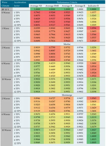
To answer research questions four and five, all simulations as listed in Table 1 will be performed. The number of tides simulated per year is related to the acceleration factor applied. To compare the bottom development of the many long-term simulations that will be performed, several cross sections will be defined which are of interest for this study. Looking at cross sections can reveal small differences between the bottom developments of the different simulations very easily. In addition, in making figures, many results for a particular cross section can be visualized in only one plot. Visualisation in this way of the performed simulations is much more efficient than comparing cumulative sedimentation and erosion patterns. For the defined cross sections, several performance indicators to quantify the accuracy will be calculated. These performance indicators are calculated with respect to the brute-force simulation of ten years and averaged over all cross sections for a quick comparison. The performance indicators include the NS coefficient, RMS, linear correlation coefficient and the slope of the linear regression line (B). An acceptable accurate result is obtained when the NS is above 0.95, the RMS lower than 0.5, R over 0.99 and B lower than 1.05. The performance indicator NS and the linear correlation coefficient (R) do have an upper limit of one (perfect match). The RMS has a lower limit of zero (perfect). These indicators are therefore easy to compare using colour scales. The optimal result for the slope of the linear regression line between the long-term accelerated simulations and the brute-force simulation of ten year is one. These results however can be both higher and lower. A colour scale is therefore not suitable. To make a colour scale possible, an upper or lower limit is needed. Therefore, an indicator for the slope of the linear regression line will be calculated. This indicator is defined as: ABS(average RMS – 1) +1. ABS means absolute value. Now the lower limit of the slope of the linear regression line is one (perfect) and a colour scale is applicable as well.
weighting the bottom development in Mormerge). Also the sedimentation and erosion of adjacent dry cells has been set to 25 % of the wet cells. These settings have been applied to all long-term simulations, including the brute-force simulations.
Table 1 - Long term simulations. For the tide-only case and the inclusion of one wave class, Morfac = Mormerge. The number of tides simulated per year in the table is related to acceleration factor applied.
Waves 0 1 2 6 10 2 6 10
Tides simulated per year
Mormerge Morfac
1 2 4 6 12
All simulations listed in Table 1, including the brute-force simulations, will start directly after the validation of the input reduction. The results of the long-term simulations are presented in section 6. During the computation of the long-term simulations, the framework for comparing the acceleration methods with the brute-force simulation will be defined (section 7). By using this framework, the distinguishing elements that decide which acceleration method and factor are most appropriate for a particular simulation will become clear (research question seven). To compare the resulting bathymetries of all simulations, bottom changes as well as sediment transport rates can be used. In this study bottom changes will be used which will result in a higher correlation coefficient compared to a reference situation as pointed out by Van Rijn (2012).
The comparison of the (sub) variants will take place by means of a Multi-Criteria Analysis. The sub-variants are simulations in which parameters as the number of tides being simulated, which is related to the acceleration factor, are varied. In the analysis, both acceleration methods including the various input conditions are compared based on predefined criteria. The assessment criteria of the different acceleration methods are: accuracy, simulation time, ease of use and applicability for a particular situation (physical justification). In engineering practice and consultancy where a project has to be finished in time because of a deadline set by the client, a simulation time of 100 - 120 hours (± 5 days) still is acceptable. Ideally for long-term simulations, a simulation time of ± 60 hours is desired. When a computer needs 60 hours to compute the final model result, approximately three simulations a week can be performed and checked if the model simulated correctly. In consultation with the supervisors of this thesis a weighting for each criterion in the MCA will be determined. The outcomes of the MCA will determine which method is most suitable for a specific situation and which elements are relevant to obtain accurate results.
2
Study area
2.1
INTRODUCTIONIn this section, the study area and field data characteristics are described. As explained in the methodology sub-section (1.3), the coastal and offshore area of IJmuiden the Netherlands is chosen as the study site for this research. The description of the field data characteristics will reveal the hydrodynamic elements of the natural system that should be included in a model to simulate the area well. These important hydrodynamic elements will form the answer to research question one; which input conditions should be combined into ‘input scenarios’ to run morphological simulations that represent the reality.
2.2
STUDY AREA [image:19.595.69.533.454.712.2]The study site chosen consists of the area outside the harbour moles of the harbour of IJmuiden, the Netherlands; see Figure 2. This area will be implemented in a schematized way (section 4). The study site covers an area from the coast up to a water depth of 20 m w.r.t. NAP and tens of kilometres wide (North – South orientation).
In the study area, the IJgeul is present which is a navigational channel in the North Sea. This navigational channel connects the offshore regions with the North Sea canal (Dutch: Noordzeekanaal) to reach the harbour of Amsterdam.
2.3
CHARACTERISTICS OF TIDE AND WAVES [image:20.595.88.513.310.648.2]The morphological development of the study area is mainly determined by waves (caused by wind) and the tide. These processes are necessary to derive input conditions for the morphodynamic development in this case study. Both processes are described more extensively in this section. Wind data is implicitly taken into account by the waves; the measured wave heights are caused by wind. In the model, no wind forcing is used to avoid wind driven currents. Field data of the tide and waves are obtained from live.waterbase.nl, the database of Rijkswaterstaat (Rijkswaterstaat, 2011). The most recent year with available validated data of all necessary measured variables is 2013. The data of the year 2013 are therefore used in this study. An example of measured data of the total water level, calculated tidal water level and measured wave height can be seen in Figure 3.
Figure 3 - Measured total water level (a) and calculated tidal water level (b) at station IJmuiden Buitenhaven. Measured wave height (c) at station IJmuiden Munitiestortplaats (Rijkswaterstaat, 2013).
2.3.1
TIDEaround amphidromic points. The propagation of the tide near the Dutch coast is therefore from South to North. The further away from an amphidromic point, the higher the tidal range usually is. The interaction of constituents (M2 and S2) and the M2 with higher harmonic M4 respectively cause the spring-neap tidal
cycle and the daily inequality of the tide in the North Sea.
For IJmuiden, the mean high vertical tide is around 1 m NAP, with spring tides up to 1.4 m NAP. The tidal range in the North is smaller than in the South, as shown in Figure 4. This difference in tidal range is caused by the position of the Netherlands with respect to the nearest amphidromic point. In addition, the tidal curve in the North Sea is asymmetrical. This is mainly caused by the distortion (phase differences) of the M2 tidal constituent by the M4 constituent, which results in a faster rise of the tide then fall (Elias, 2006).
Figure 4 - Tidal range (in cm) along a part of the Dutch coast measured from Den Helder (0 km) (Van de Rest, 2004), data from (RIKZ, 2003). Red lines are indicating mean high water and mean low water for locations along the Dutch coast.
2.3.2
WAVES3
Morphological acceleration
techniques in numerical modelling
This section describes the morphological acceleration techniques Morfac and Mormerge. Besides input reduction, to be discussed in section 5, an acceleration of the morphological changes is an approach frequently applied to accelerate the morphodynamic long-term computations. In this section, first an introduction is provided in which a morphodynamic loop is shown and what in general the acceleration methods do. Next, the different acceleration methods will be discussed including the way they will be used in this study.
To compare the acceleration methods, a reference simulation will be performed. This reference simulation, called a brute-force simulation, uses a reduced tidal signal and a real-time wave signal without an extra acceleration of the morphological changes (because of the good applicability of this tide, see section 5.1). The brute-force simulation is performed for one year and will be compared to the same brute-force simulation, however accelerated with a factor ten to account for ten years (time span of long-term simulations). The comparison will be done when both brute-force simulations simulated one year of morphodynamic development. This comparison is done in order to check the performance of the ten year brute-force simulation compared to a non-accelerated simulation (further explained in section 6.1). In addition, various acceleration factors are tested in this case study. For both acceleration techniques, the acceleration factors applied are multiples of the number of harmonic morphological tides simulated per year (result of the input reduction as will be executed in section 5). Questions as: which equations are solved and in what sequence will be answered in this section. Also the implementation of the methods in Delft3D and the physical meaning of different elements will be provided. In the end, the similarities and differences between the acceleration methods and their implementation in Delft3D will become clear.
3.1
INTRODUCTIONMorphological models are indispensable tools for simulating the morphological behaviour of coastal areas, river- and sea bottoms. These models make use of a hydraulic-morphological system, or morphodynamic cycle, to calculate flow, sediment transport and bottom changes (Ribberink, 2011). The morphodynamic cycle can be tidally averaged, intra-tidal or by another user specified preferences be calculated. An example of a morphodynamic cycle is shown in Figure 6. Other, but similar examples of morphodynamic cycles can for instance be found in Ribberink (2011), Roelvink (2006) and Wijnberg (1995).
The morphological acceleration techniques accelerate the computation in various ways. The methods are developed on progressive insight in morphological modelling and computational power. Because of the progressive insight in morphodynamic accelerated modelling and the fact that all recently performed studies in this field use the Morfac or Mormerge method, the emphasis in this thesis is on these methods. The governing equations that are solved during the computation in Delft3D can be found in Appendix A: Delft3D model description.
Figure 6 – Example of a morphodynamic loop, or cycle
3.2
MORFACMorfac is the first method that is characteristic for running flow, sediment transport and bottom updating all at the same small time steps. This contrasts previous methods for morphological acceleraction. Morfac is adapted from the elongated tide concept by Latteux (1995). The literature around this new method started around 2003 – 2004 when Lesser et al. (2004) proposed a three-dimensional morphological model with an morphological acceleration factor to accelerate the morphological changes for long-term modelling. The computation of the different components simultaneously and the two-way interaction of the flow and waves in which the sediment transport is calculated instantly, make it easy to include interactions between flow, sediment and morphology. This also reduces the storage of large amounts of data between the different processes (Roelvink, 2006).
The approach of running the flow, sediment transport and bottom updating at the same time does not take into account the difference between the morphodynamic and the hydrodynamic time-scales. To take advantage of this, a factor n is used to accelerate the morphological depth changes . In Delft3D, this multiplication is applied to the net sediment transports (bed load and/or suspended load) which are calculated every half time step (in water level points and half a time step later in the velocity points). The depth change based on the net sediment transports can be caluclated, if desired, every half a time step too. In order to avoid the violation of the continuity of sediment mass in the model, expressions are included that limit the erosion if the quantity of sediment at the bed approaches zero (Lesser et al., 2004). It is therefore important to check the thickness of the sediment layer in the model regularly.
A difference with previously used acceleration methods is that the bottom changes are computed in much smaller time steps. With a Morfac of 60, approximately one year of morphological change is simulated after 12 tidal cycles. If in a flow model, a time step of 5 minute is used, with a morfac of 60 the bathymetry is still updated every five hours. This results in a significant reduction of the computational time for Morfac. However, the short-term changes in reality due to varying wave and tide interactions put a limit on the morphological factor that is usable in simulations. A way to overcome this problem is to use a morphological factor that varies depending on the wave conditions. This is called variable Morfac. In this variant of Morfac, severe storms with a relatively low probability of occurrence would have a small Morfac and normal everyday conditions a high Morfac. The defined combinations of particular wave conditions with the tide, based on the input reduction as will be executed in this study, are simulated separately in a random sequence using the bottom layout of the previously executed class. All conditions are summed based on their percentage of occurrence or by changing the simulation times per condition (Lesser, 2009).
In this study, the time to be simulated is kept the same for all conditions. All conditions will be simulated for 10 years. Including a variable morfac (acceleration factor * percentage of occurrence of a particular wave condition) makes sure that every wave condition produces the right amount of morphological development, see Figure 8. The acceleration factors are choosen such that an integer number of harmonic morphological tides (result of the input reduction to be applied in section 5.1) are simulated per year as explained at the beginning of this section.
Figure 7 - Flow diagram of Morfac with an acceleration factor n
3.3
MORMERGEAnother method that has the stability and rate of accuracy of Morfac, but can perform the computations parallel, is Mormerge (Roelvink, 2006). In this approach it is assumed that the hydrodynamic conditions vary much more than the morphology. If the time interval in which all hydrodynamic conditions occur (ebb, flood, spring tide, neap tide, storms etc.) is small compared to the morphological time-scale, these processes can be run in parallel, using the same bathymetry and same acceleration factor for all conditions. This bathymetry is subsequently updated using a weighted average of the sediment transport rates for all hydrodynamic conditions based on the occurrence of the wave classes. The flow scheme of the method can be seen in Figure 9.
The various parallel processes for flow, wave and sediment transport can be defined based on different conditions that are present in a study area. These processes (input conditions) in this study are derived by applying input reduction (section 5). By computing the processes parallel, it is possible to include an instantaneously counteraction of conditions as is in reality. An example is that other tidal phases can be assigned to different wave conditions. This will lead to ebb and flood sediment transports counteracting each other at all times (as most times in reality) and can allow for the use of much higher morphological acceleration factors because of the reduced short-term amplitude changes (Roelvink, 2006). The tidal phase shift applied in this study is equally divided over the number of conditions included. A particular phase shift is randomly assigned to a wave class. For example, performing a Mormerge simulation which includes 10 wave classes, a phase shift per wave class of 36° (360°/10) is applied.
Figure 9 - Flow scheme of Mormerge with an acceleration factor included n included for all conditions.
For Mormerge, the bathymetric changes are weighted every flow time step. The weights in this study are a result of the input reduction for the waves as will be performed using the OPTI-routine. OPTI weights for the wave classes summed do not necessarily have to be equal to one. Because Mormerge automatically scales the OPTI weights to one, care should be taken to extract the correct output which represents a ten yearly morphodynamic development).
3.4
SIMILARITIES AND DIFFERENCES OF MORFAC AND MORMERGEby an acceleration factor to determine the new bathymetry. This new bathymetry, computed every time-step, ensures that the hydrodynamic flow calculations (and waves) are always executed using the correct bottom layout.
4
Model setup
4.1
DELFT3D PROCESS-BASED MODELTo simulate the long-term morphology of the study area, the process-based model Delft3D is used (in 2DH mode, Open Source version 4168). This model describes waves, currents, sediment transport and bed level changes by a set of mathematical equations based on the conservation of mass, momentum, energy, etc. Delft3D consists of several modules of which two of them, the FLOW-module and the WAVE-module, are used in this thesis. The FLOW-module is the central module which communicates with the WAVE-module. A general overview of the equations solved in Delft3D and the solving scheme is given in Appendix A. This section describes the numerical input as the grid, initial bathymetry, physical parameters and other settings, boundary conditions and initial conditions.
4.2
GRIDThe grid used in this study is an orthogonal curvilinear staggered grid. This grid is constructed using the RGFGRID feature of Delft3D. When constructing a grid, attention should be paid to the features that have to be modelled. Important areas and processes need to have sufficient grid cells to represent that particular item well. Furthermore, some general guidelines for constructing a grid are determined by Arcadis (Grasmeijer, Adema, & Jellema, 2014). These guidelines are restricting the maximum smoothness in both directions, the orthogonality and the aspect ratio. The smoothness is the ratio between the lengths of adjacent grid cells in a certain direction. The orthogonality determines the perpendicularity of a cell and the aspect ratio is the ratio between the length and the width of a grid cell.
In this research, a schematized study area of the coast of IJmuiden is chosen (see section 2, Study area). The schematization of the study area compared to the reality can be seen in Figure 10. The grid approximately is 15 * 42 km (M*N direction, see Figure 10). The other important characteristics of the grid and the grid criteria for a Delft3D computation are listed in Table 2.
Table 2 - Grid characteristics
Grid Criterion (Grasmeijer, Adema, & Jellema, 2014)
Total number of cells 21624 -
M number of cells 106 -
N number of cells 204 -
M –smoothness 1.13 < 1.2
N – smoothness 1.19 < 1.2
Orthogonality 0.006 < 0.04
To model the nearshore processes and the behaviour of the nautical channel accurately, the grid has been refined in these areas of interest. The coarsest grid cells at the boundaries are 450 * 300 m (M*N direction). The finest grid cells in- and around the nautical channel and the coast are 30 * 15 m (M * N direction).
Figure 10 - Grid study site, coastal area IJmuiden. With real land boundary (red) and schematization (black)
4.3
NUMERICAL PARAMETERS4.3.1
INITIAL BATHYMETRYThe initial bathymetry used in this study is constructed with the Quickin feature of Delft3D. This initial bathymetry is derived from JARKUS Raaien profiles in the area of interest. The Raaien 4800, 5000, 6000 and 6200 are assumed to represent an average uniform coastal profile around the harbour moles of IJmuiden, see Figure 11. From these profiles, the average coastal profile of IJmuiden has been derived. The average profile for the initial bathymetry starts at +5 m NAP to make sure that under the tidal elevation and wave height, no reflective numerical processes at the coastal boundary will occur in Delft3D. The average coastal profile has been extended with an exponential slope to -20 m NAP at 15 km offshore the coast, see Figure 11.
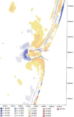
In the study area grid and initial bathymetry, the IJgeul is present (a nautical channel) that is around 20 m deep. This nautical channel is enclosed by harbour moles in the nearshore. The harbour moles are represented by thin dams in Delft3D that reach up to approximately 1200 m offshore where the water depth approximately 9 m is. Thin dams are chosen because these features are much smaller than the grid cell size. The bathymetry including the harbour moles and the nautical channel is shown in Figure 12. The bathymetry is very similar (but more schematized) to the bathymetry used in a study to reduce the sedimentation between the harbour moles (Bijlsma, Mol, & Winterterp, 2007).
A A’
B’
Figure 11 - JARKUS profiles of Raaien 4800, 5000, 6000 and 6200 in 2013 (Rijkswaterstaat, 2013).
4.3.2
BOUNDARY CONDITIONSThe numerical model Delft3D used in this study can solve the hydrodynamic and morphodynamic calculations with various boundary conditions. Which type of boundary conditions is most suitable, depends on the phenomena to be studied and the information available in the study area (Deltares, 2014).
For this study, several measuring locations are present in, or nearby the study area. To convert data from these stations to the exact location of the boundary conditions, interpolation of data from at least three stations is needed. To avoid this cumbersome interpolation of all boundary segments of the model, the model has been nested into an overall model, the Kuststrookfijn Astro model (abbreviated as Kustfijn) developed by Arcadis2 (Alkyon, 2001b). The Kustfijn model has been validated to reproduce water levels at the Dutch coast. An example of the model domain of the Kustfijn model including the study area of this thesis is shown in Figure 13.
The open boundaries (North, West and South) of the nested model are divided into segments. The East boundary (the coast) is a closed boundary. This closed boundary is an upsloping beach to 5 m + NAP which can flood and dry. The start and end points of the open boundary segments are extracted from the overall model. To match the boundaries of the nested model as closely possible with the overall model, a maximum of 5 grid cells per segment is applied. This makes that the North and South boundaries are both divided into 21 segments and the West boundary into 41 segments. Between the start and end point of the segments where the water level is extracted from the overall model, the intermediate points are linearly interpolated. For the WAVE module, the same boundary locations are applied except that these boundaries are uniform (no subdivision into segments). The imposed wave conditions are the same for all boundaries and are uniformly applied over the boundaries. The wave boundaries nearshore are left out to avoid unrealistically high waves at the coast (H = 0 up to approximately 10 m water depth).
Figure 13 - Model domain Kustfijn model including the enclosure of the study area
Because of the validated water levels of the Kustfijn model, a water level boundary condition has been chosen for the Western boundary of the study area. It is however not desirable to include all boundaries of
the type water level. A small error in the water levels will result in continuity problems. These continuity problems can only be compensated for in a large response of the velocity components (Deltares, 2014). Therefore, at the cross-shore boundaries (North and South) a Neumann type of boundary condition is applied. This type of boundary condition specifies the normal water level gradient. In combination with the Western water level boundary, the solution of the mathematical boundary problem is well-posed. The Neumann boundary conditions at the cross-shore boundaries can handle various different processes acting on a boundary where the exact water level or velocity is not known beforehand, as is desired in this study. Using this type of boundary, the model determines the correct solution for the Neumann boundary segments by applying the imposed normal water level gradient (Roelvink & Walstra, 2004).
To avoid the model making an artificial boundary layer along the boundary, the advective terms containing the normal gradients of the open boundaries are switched off. In addition, the water level boundary is made less reflective. The reduced reflection makes sure that short wave disturbances propagating towards the boundary from inside the model are not fully being reflected back into the domain as is the case when this parameter is set to zero.
4.3.3
OTHER PARAMETERS AND SETTINGSThe sediment concentration used in this study contains only one fraction. The D50 of this fraction is 200 µm
with a specific density of 2650 kg/m3 and a dry bed density of 1600 kg/m3. This D50 value is found
representative for the study area (Van Alphen, 1987; Wijnberg, 1995). A uniform Chézy roughness coefficient of 65 m1/2/s and a horizontal eddy viscosity of 1 m2/s are used in the model (default Delft3D).
The water density has been set to 1020 kg/m3. In the model, no salinity or temperature gradients are
included.
To calculate the flow, a hydrodynamic time-step has to be specified which fulfils the Courant number criteria. This criterion provides an indication of the accuracy and numerical stability of the model and should generally not exceed a value of ten. For an implicit scheme where stability is not an issue (as is used in this study), the Courant number criterion is mainly important for the accuracy of the model. The Courant (Friedrich-Lewy) number (CFL) criterion for Delft3D is defined as (Deltares, 2014):
𝐶𝐹𝐿 = ∆𝑡 √𝑔𝐻
min {∆𝑥, ∆𝑦}< 10 → ∆𝑡 <
10 ∗ min {∆𝑥, ∆𝑦}
√𝑔𝐻 =
10 ∗ 15
√9.81 ∗ 20= 10.7 𝑠 1 In which ∆𝑡 is the time step (in seconds), g the acceleration of gravity (m/s2), H the maximum water depth
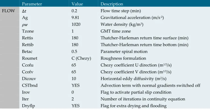
(m) and 𝑚𝑖𝑛{∆𝑥, ∆𝑦} is the minimum of the smallest grid sizes (m). For this study, the minimum of the grid cells is approximately 15 m and the maximum water depth is 20 m in the nautical channel. This results in a maximum time step of 10.7 sec. Because of the relatively simple geometry of the model, a time step of 12 seconds (0.20 minutes) is applied. This small violation of the CFL criterion does not result in a decreased performance in terms of accuracy (section 5.3). The frequency of the communication between the FLOW and WAVE modules in Delft3D is set to 60 minutes. The measurement interval of the wave climate used is also 60 minutes. A complete list of all parameters used in the model can be found in Appendix A.6.
4.3.4
INITIAL CONDITIONS5
Input reduction
In simulating the medium- and long-term morphodynamic behaviour of a study area, input reduction is desirable to avoid unnecessary time consuming computations with real-time data (Latteux, 1995). This input reduction will be applied to the tide and wave boundary conditions. Afterwards, the simulation results of the reduced input conditions are validated based with a simulation using real-time data (no input reduction). This section will provide an answer to research question three in what way a tidal signal can be reduced to a representative tide for an accurate long-term simulation.
5.1
TIDE SCHEMATIZATIONFor the schematization of the tide, a so called ‘morphological tide’ will be derived. This morphological tide is a harmonic tide of two consecutive tidal cycles that should result in the same morphological development as a daily average of the astronomical tide for approximately a full spring-neap tidal cycle. The morphological tide will be chosen such to match the change in the morphology for an entire spring-neap cycle in reality as closely as possible. Because of the daily inequality of the tidal water levels in the study area, a double morphological tide (or two consecutive tides) will be derived.
In this study the method of Roelvink & Reniers (2012) is used which is in principle the same as Latteux (1995). Roelvink & Reniers (2012), however, recommend to only calculate one spring-neap tidal cycle instead of a full year of morphological behaviour to derive the morphological tide. The method is easy to apply and uses a scaling factor directly derived from linear regression instead of a calibration of parameters such as in the method of Lesser (2009). The following procedure should be executed to derive the morphological tide according to Roelvink & Reniers (2012):
First, a simulation of flow and sediment transport including bottom changes over approximately a full spring-neap tidal cycle should be performed as a reference situation (simulation without waves).
The next steps has to be performed for each consecutive tide (double tide in this study):
1. Calculate the correlation between the tide-averaged transport rates or bottom changes in all grid points for the full spring-neap tidal cycle and all consecutive double tides separately. The linear correlation coefficient is defined as:
𝑟 = 𝑐𝑜𝑣(𝑥, 𝑦)
𝜎(𝑥) ∗ 𝜎(𝑦) 2
2. Together with the correlation coefficient, the slope of the linear regression line between the bottom changes of the full spring-neap tidal cycle and each double tide has to be calculated. This slope parameter indicates the correctness of the magnitude of the bottom changes; a slope equal to the number of double tides simulated is a perfect match. This slope parameter is used as a time-scale factor. The computed bottom changes should be multiplied with this factor to obtain the actual bottom changes for a full spring-neap tidal cycle.
Both parameters, the correlation coefficient and the slope of the linear regression line combined provide quantitative information of the shape and magnitude of all double consecutive tides in which they represent the shape and magnitude of bottom changes of the simulated spring-neap tidal cycle. Ideally, a double tide should be chosen with a correlation coefficient closest to one and a slope parameter closest to the number of double tides simulated.
For this study, the following parameters are calculated for the approximately simulated spring-neap tidal cycle (2/4/2013 to 30/4/2013, 28.45 days), see Figure 14 (here only the best fit of all tides is shown, the results of the other double tides can be found in Appendix B.1). From the full series, the tide with the highest correlation and the most adequate slope parameter is no. 20 (Figure 14). This tide has a correlation coefficient of 0.9993 and a slope parameter of 20.342. This tide is visualized in Figure 15. The tide period is from 11 April 2013 06.50 h to 12 April 2013 07.40 h and is chosen as the morphological tide for this study. The morphological development (cumulative sedimentation and erosion pattern) of this full spring-neap tidal cycle can be seen in Appendix B.2.
Figure 14 - Correlation and slope parameter of morphological tide
To make the selected tide a perfectly periodic boundary condition with a base frequency equal to the M2
tidal constituent frequency, a harmonic analysis of the selected time series is performed. For this harmonic analysis, the selected morphological tide is repeated several times to be able to extract various harmonic constituents from this signal. The main tidal constituents derived from this signal are the M2 and higher
harmonics M4, M6 and M8 tidal constituents. Amplitudes and phases values of the harmonic tidal
constituents for the grid corner points northwest and southwest are listed in Table 3. The choice for only incorporating these four constituents is supported by the tidal form factor F which is defined as (Pugh, 2004):
𝐹 = 𝜁̂𝐾1 + 𝜁̂𝑂1
𝜁̂𝑀2 + 𝜁̂𝑆2= 0.14 3
This value of 0.14 means that the tide is semidiurnal and thus mainly determined by the M2 constituent
distorted by the higher harmonics. The derived harmonic morphological tide is shown in Figure 16. The derived harmonic morphological tide shows the characteristics of the increasing tidal amplitude towards the South and towards the coast as expected by the explanation of the characteristics of the tide in the North Sea (section 2.3.1).
Table 3 - Harmonic tide conditions
Location Constituent Amplitude (m) Phase (°)
Northwest M2 0.6624 142.90
M4 0.2213 178.27
M6 0.1115 239.92
M8 0.0613 303.66
Maximum total amplitude 1.0565
Southwest M2 0.7138 99.53
M4 0.2804 151.84
M6 0.0477 214.41
M8 0.0546 212.15
Maximum total amplitude 1.0965
5.2
WAVE SCHEMATIZATIONA full wave climate is the state of the waves at a certain location over a period of time. These conditions depend on meteorological conditions and can vary from time to time (even from second to second). In practice, it is impossible to include all these short variations. Therefore, a schematization of the wave climate is necessary. Regarding the schematization of a full wave climate, as for example shown in Figure 3c, the goal is to reduce the wave classes as much as possible without losing much accuracy in the morphological development of these waves compared to the full wave time series.
The schematization of the wave climate will be done for the characteristics of the waves measured at the ‘’IJmuiden munitiestortplaats’’ measurement location. It is located around 30 km offshore in front of IJmuiden where the water depth is around 20 m (Van de Rest, 2004), equal to the water depth at the seaward open boundary of the model used in this study. The measured wave characteristics are therefore assumed to give representative values at the boundaries of the model used in this study.
To schematize the wave climate, the time series of the year 2013 is used to take the hourly, daily, weekly and even seasonal variations into account. These wave conditions in turn are classified into directional and magnitudinal classes, as can be seen in Figure 5. The full wave climate is divided into 12 directional and 12 magnitudinal classes and thus into 144 different combinations of wave height and direction. However, because of the location of the measurement station (far offshore), the waves occurring from 15° to 195° w.r.t. North (measured clockwise), are not realistic in this study. These waves would then originate from the land. Leaving out these waves leaves 72 combinations. In addition, not every combination of wave height and wave direction is present (see Figure 5). This results in 62 combinations of wave height and wave direction for this study area. All combinations are listed in Table 12, Appendix B.3).
The full wave climate divided into 62 distinct classes will now be reduced to scenarios with 0, 1, 2, 6 and 10 different wave classes to compare the morphological acceleration methods. All those scenarios should reproduce the full wave climate as closely as possible. To select the best combinations of classes, two frequently used approaches exist (Van Rijn, 2012):
The first approach is to manually determine the wave classes based on the wave height, direction and morphological impact. The morphological impact is assumed to be proportional to the wave height to some power and is derived from the CERC formula for alongshore sediment transport at a uniform coastline.