Frequency optimisation for damage identification using the Vibro Acoustic Modulation method

(1)

Faculty of Engineering Technology

Research group Dynamics Based Maintenance

Frequency optimisation for

damage identification using the

Vibro-Acoustic Modulation

method

Master Thesis

M. Venterink

s0190853

Date:

January 20, 2017

Examination committee:

prof. dr. ir. T. Tinga dr. ir. R. Loendersloot ir. J.S. Hwang

ir. J.P. Schilder

Document Number:

(2)

(3)

Preface

This report is the result of my research for the Master Degree in Mechanical Engineering at the University of Twente. My master program in the faculty of Engineering Technology started by the chair Applied Mechanics but my final master assignment was carried out by the Dynamics Based Maintenance group.

Without the help of my supervisors it would not have been possible to finish my thesis. Richard Loendersloot and Jason Hwang helped me with their critical comments and insightful advises throughout my graduation project. Our discussions kept me going and I am very thankful for that. Not to forget Tiedo Tinga for his comments and advises. Then I would like to thank Axel Lok for his help on my experimental setup and Gert-Jan Nevenzel for the production of the composites plates at TPRC. Furthermore I would like to thank my fellow students from the ‘MS3Bazen’ room for the occasionally useful discussions and ofcourse the pleasant times.

Finally I would like to thank my family and friends for their support during the difficult times in 2016. Especially my girlfriend Pauline who has supported me to finish my master assignment and achieving my cycling goals at the same time.

Januari 2017, Enschede Martijn Venterink

(4)

(5)

Summary

Composite aerospace structures are desired to have an extended service life and a reduction of maintenance costs without compromising safety. The presence and severity of possible damage has to be monitored to guarantee safety. Aerospace structures are especially sensitive to im-pact damage that results mostly in delaminations. The steady state Vibro-Acoustic Modulation (VAM-)method has shown to be a promising non-destructive technique for damage identification in a composite structure using two excitation frequencies: a low intense pump frequency (mostly a natural frequency) and a relative weak and high carrier frequency. Research on the influence of the carrier frequency selection, which is mostly done arbitrary, on the response signal modu-lations is however limited.

The main objective of this graduation assignment is to achieve an ideal combination of a pump and carrier frequency for a more efficient damage detection, localization and characterization on a composite with a delamination. The secondary objective is to explain the occurring signal modulations for different carrier frequencies.

Analytically derived nonlinear dynamic responses of a multi degrees of freedom system subjected to a two-tone forced harmonic, show the relation of amplitudes of the carrier, pump, higher har-monics and sidebands with the natural frequencies. These natural frequencies are separated into the global natural frequencies of the composite plate structure and the local natural frequencies of the delamination. The global and local eigenfrequencies of the composite plate are determined numerically such that the dimensions of the manufactured composite plate and its artificial de-lamination can be chosen.

Experimentally, the natural frequencies of the produced composite plate are also determined and a separation between local and global is made. The pump excitation with the expected clapping behavior that causes the most signal modulations is selected for the VAM-experiments, i.e. the delamination shows an opening and closing behavior by the operational deflection shape of the pump excitation. Finally the carrier frequency is varied with a constant carrier excitation amplitude.

Firstly, the VAM-method promises to be more effective in damage detection and localization when using a local natural frequency as the carrier. The modulations will increase more in the damaged location than in the undamaged location compared to using a global natural frequency as carrier. Secondly, the frequency modulation for varying carrier frequencies has shown to be very inconsistent. Therefore it is concluded that damage localization with amplitude modulation in the time domain is better than using the sidebands in the frequency domain, because sidebands are a function of both amplitude and frequency modulation. Finally, a framework has been considered for a practical application of VAM.

(6)

(7)

Samenvatting

Voor composiet structuren in de vliegtuigindustrie is het gewenst om een langere levensduur en een reductie van onderhoudskosten te hebben. De veiligheid mag niet in gevaar komen en daarom moet de aanwezigheid en heftigheid van mogelijke schade constant in de gaten gehouden worden. Composieten kunnen interne schades hebben die aan de buitenkant nauwelijks of niet zichtbaar zijn. Een delaminatie tussen twee lagen is een veelvorkomende schade in de vliegtuigin-dustrie ten gevolge van impact schade. De Vibro-akoestische modulatie (VAM-)methode is een veelbelovende niet-destructieve test techniek om zulke schade te identificeren in een composiet. Deze methode maakt gebruik van twee excitatie frequenties, een sterke en lage ‘pomp’ frequentie (meestal gelijk aan een eigenfrequentie) en een relatief zwakke en hoge ‘dragende’ frequentie. Het effect van de keuze van de dragende frequentie op de signaal modulaties is echter nog maar weinig onderzocht.

Het hoofddoel van deze afstudeeropdracht is om een betere combinatie van een pomp en dra-gende frequentie te vinden om zo een effici¨entere schade detectie, lokalisatie en karakterisatie te krijgen voor composieten met een delaminatie. Een subvraag van dit hoofddoel is het verklaren van de optredende signaal modulaties voor verschillende dragende frequenties.

Niet-lineaire dynamische responsies zijn analytisch afgeleid van een systeem met meerdere vri-jheidsgraden die met twee harmonische krachten ge¨exciteerd wordt. Deze responsies tonen een relatie aan tussen de amplitudes van de pomp, de dragende, de hogere harmonische en de zoge-naamde ‘sidebands’ met de natuurlijke frequenties van het systeem. Deze natuurlijke frequenties zijn vervolgens opgesplitst in de globale natuurlijke frequenties van de composiet plaat en de lokale natuurlijke frequenties van de delaminatie. Deze globale en lokale eigenfrequenties zijn eerst numeriek bepaald om zo vervolgens de afmetingen van de te maken composiet plaat en de bijbehorende delaminatie te kunnen bepalen. De daadwerkelijke natuurlijke frequenties van de geproduceerde plaat zijn vervolgens experimenteel bepaald, en een onderscheid is gemaakt tussen lokale en globale frequenties. Een pomp frequentie is vervolgens geselecteerd die het verwachte open en sluiten gedrag van de delaminatie veroorzaakt en die de meeste signaal modulaties veroorzaakt. Tot slot is de dragende frequentie gevarieerd met een constante excitatie amplitude.

Ten eerste is er geconcludeerd dat de VAM-methode effici¨enter in het detecteren en lokaliseren van schade is wanneer er gebruik wordt gemaakt van een lokale natuurlijke frequentie als dra-gende frequentie. De signaal modulaties zullen heftiger zijn in het beschadigde gebied dan in de onbeschadigde gebieden. Ten tweede is er geobserveerd dat de frequentie modulatie voor verschillende dragende frequenties erg inconsistent is ten opzichte van de amplitude modulatie. Daarom is er ook geconcludeerd dat schade identificatie door middel van amplitude modulatie in het tijdsdomein beter is dan gebruik te maken van de zogenaamde ‘sidebands’ naast de dragende frequentie in het frequentie domein. Ten slotte is er een stappenplan gemaakt aan de hand van de resultaten in dit onderzoek, zodat VAM ook in de praktijk toegepast kan worden.

(8)

(9)

Nomenclature

The Greek and Roman symbols, and the abbreviations used in this master thesis are categorized. Some symbols can represent multiple quantities, the exact meaning follows from the textual context. An overview of the most important abbreviations and symbols used in the present thesis is:

Abbreviations

AM Amplitude modulation

BVID Barely visible impact damage

C Clamped

DOF Degree(s) of freedom

FFT Fast Fourier transform

FM Frequency modulation

FRF Frequency response function

HT Hilbert transform

NDT Nondestructive testing

NLR National aerospace laboratories

ODS Operational deflection shape

PM Phase modulation

PZT Piezo-electric transducer

SHM Structural health monitoring

SS Simply supported

VAM Vibro-acoustic modulation

Greek symbols

βAM Amplitude modulation index [-]

βF M Frequency modulation index [-]

Control factor for the nonlinear function [-]

ν Poisson’s ratio [-]

ρ Density [kg/m3_]

φinst Instantaneous phase [rad]

φp Phase of the pump excitation signal [rad]

φc Phase of the carrier excitation signal [rad]

ω Frequency [rad/s]

ωp Frequency of the pump excitation signal [rad/s]

ωc Frequency of the carrier excitation signal [rad/s]

ωo Natural frequency [rad/s]

ωinst Instantaneous frequency [rad/s]

(12)

Roman symbols

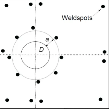
a Distance between delamination and weldspot [mm]

Ac Carrier amplitude [m]

Ap Pump amplitude [m]

Asb1 Left sideband amplitude [m]

Asb2 Right sideband amplitude [m]

Ainst Instantaneous amplitude [mm/s]

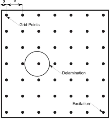
d Distance between grid-point and edge [mm]

D Delamination [-]

e Distance between grid-points [mm]

E Young’s modulus [N/m2_]

Fc Excitation carrier amplitude [N]

Fp Excitation pump amplitude [N]

f Frequency [Hz]

fres Resolution frequency [Hz/bin]

fc Carrier excitation frequency [Hz]

fp Pump excitation frequency [Hz]

fs Sampling frequency [Hz]

finst Instantaneous frequency [Hz]

fn

global Global natural frequency [Hz]

fn

local Local natural frequency [Hz]

HF v Frequency response function (mobility= velocity/force) [(mm/s)/N]

HV v Frequency response function (mobility= velocity/Voltage) [(mm/s)/V]

H Thickness of the plate [mm]

H2 Thickness of the delamination [mm]

Jn Bessel function of the first kind [-]

L Length of plate [mm]

L1 Length to delamination [mm]

L2 Length to delamination [mm]

Ma Amplitude modulation [mm/s]

Mf Frequency modulation [Hz]

m Mass [kg]

n Number [-]

q Displacement vector [m]

qbp Bandpass filtered displacement response [m/s]

R Delamination radius [mm]

SF v Cross-power spectral density (force - velocity) [(Nmm/s)/Hz]

SV v Cross-power spectral density (voltage- velocity) [(Vmm/s)/Hz]

SF F Auto-power spectral density (force - force) [V2/Hz]

SV V Auto-power spectral density (voltage - voltage) [N2/Hz]

t Time [s]

V Voltage [V]

vvp Bandpass filtered velocity response [m/s]

(13)

Chapter 1

Introduction

The selection criteria for using composites is to obtain a lighter and stiffer construction. Nowa-days, composite structures are also desired to have an extended service life and a reduction of maintenance costs [1]. These demands contradict each other, making it difficult to get an optimal solution. A disadvantage of using composites is that the structure is more prone to (impact-)damage [2]. Non-destructive testing (NDT-)techniques are a promising technique for damage detection, especially Structural Health Monitoring (SHM). It has the potential to reduce maintenance costs because some SHM techniques are capable to detect damage early on in spe-cific circumstances. The development of these SHM techniques are a widely discussed topic in the literature. They have mainly been applied to very different structures and this makes it very hard to compare all the different techniques. The Vibro-Acoustic Modulation (VAM-)technique shows to have great potential. Different VAM-methods already exist and one will be the topic of this thesis.

1.1 Composite structures

Composites are used in many lightweight engineering structures due to their high specific strength, low density and their resistance to fatigue and corrosion. Composites also have flexibility in de-sign. This flexibility allows for the production of complex shapes such as curved panels and skin-stiffener structures. Applications of composites are mostly in demanding environments, such as: wind turbines, space and aircraft structures but also high-end sports, like motor-racing and cycling. In particular the use of composites in the aerospace industry is advancing very fast, even though the application in this industry is very conservative.

A composite consists of a matrix and reinforcements. The matrix consists of a polymer when applied to aerospace structures. The reinforcement improves the composite’s overall properties but will result in anisotropic properties. Typical materials for fiber reinforcements in polymer composites are glass and carbon, but also high strength polymers such as aramid and high temperature resistant silicon-carbide could be used as fibers.

Figure 1.1: The multi-scale levels related to fiber reinforced plastics as in [3].

(14)

CHAPTER 1. INTRODUCTION

The fibers, the matrix, an individual layer and the stacked layers all behave on a different scale. The scale of the fibers and the matrix are of a lower level than the scale of an individual layer. A laminate is build from different layers and is therefore of a higher scale. The structure level is the highest level. An complete overview of these different levels is given in figure 1.1 and can be used to indicate where a specific damage can occur.

1.1.1 Damage categories

The disadvantage of using composite materials in aerospace applications is that these structures are more sensitive to damage than metals. Shock, impact or repeated cyclic stresses can cause damages to composites but also to the widely used aluminum structures. Aluminum is very sensitive to repeated cyclic stresses since it does not have a distinct fatigue limit. Composites are especially sensitive to impact damage [4]. Damages in composite aerospace structures can be categorized according to their severity [5]:

1. Allowable damage that may go undetected by scheduled or direct field inspection, for example allowable manufacturing defects, but also non-allowable damage: Barely Visible Impact Damage (BVID), e.g. caused by debris or hailstones.

2. Damage detected by scheduled or directed field inspection at specified intervals, e.g. exte-rior skin damage or inteexte-rior stringer blade damage.

3. Obvious damage detected within a few flights, e.g. accidental damage to lower fuselage or a lost bonded repair patch.

4. Discrete source damage immediately known by the pilot limiting flight maneuvers, e.g. rotor disk cut through fuselage or severe rudder lightning damage.

5. Severe damage created by anomalous ground or flight events.

The first category contains damage that can easily go undetected. The other categories all contain damage that will likely be detected by a scheduled or a direct field inspection and most of the time can be clearly visual spotted. Damages in the categories 1 to 4 have to be taken into account during aircraft design and for the damages of category 2 to 5 repair scenarios are required. The first category is the most interesting one because damage from this category is not directly harmful for the functioning of an airplane. However timely detecting damage in this category results in less maintenance costs before it expands into a severer damage category.

1.1.2 Damage types

A damage in a composite structure can have different origins. The type of damage can be categorized in the following three groups [5]:

• Accidental damage

• Fatigue damage

• Environmental damage

(15)

[image:15.595.233.390.188.279.2]

Different damage types can occur which are unknown to homogeneous materials. Failure can happen on the macro, meso and micro scales which are mentioned in figure 1.1. Delaminations, matrix breakage, debonding, fiber failure are shown to be the main failure modes of impact dam-age [2]. These damdam-age types are likely to cause severe degradation of the mechanical properties and critical failure of the part/structure if they are not discovered in time.

Figure 1.2: Schematic representation of transverse crack and delamination in a [0/90/0]s laminate [3].

A schematic representation of a delamination and a matrix crack is given in figure 1.2. Delamina-tions (with matrix cracks present) are the most discussed failures of a composite in the literature [7, 8]. Laminated composites are especially susceptible to delamination owing to their weak transverse tensile and inter-laminar shear strengths as compared to their in-plane properties.

1.1.3 Damage lay-out

Failure of composite structures is quite complex and usually involves the combination of several failure modes. All kinds of different inflicted damages on composites are discussed in the litera-ture [4]. The focus in this study will be on the high-velocity low-mass impact damage that most likely will cause BVID with delaminations. Which failure modes are present in a test-specimen depends on the technique that is used to apply the damage. An impact test will result in more realistic damage and will likely contain different kinds of failure modes over one or multiple layers [2].

An artificial damage can be created to control the damage such that only a specific failure mode is present in the specimen. For example inserting a piece of Teflon between two layers in the production process will only contain one specific delamination between two layers in the test-specimen [3, 9, 10]. If the Teflon is inserted before consolidating the structure in the autoclave, the Teflon will evaporate because of the high temperature. This artificial delamination will differ from an actual delamination. Such a real life delamination can still have fibers crossing in the delamination, the artificial delamination will not have those fibers crossing in the delamination. The shape of the delamination will be very well controllable with this technique.

Another option that can inflict damage (delamination) in a controllable situation is a three point bending loading technique. This is used in a different study to create damage in a composite plate [11]. Different loadings are used for different test-specimens. Delaminations and matrix cracks are created in each specimen with a different damage severity. This already demonstrates that the inflicted damage is not that controllable as in the previous discussed artificial delaminations.

(16)

(a) Impact energy of 2.04 J [12]. (b) Impact energy of 10.1 J [12].

Figure 1.3: Two impact tests with a different impact energy, as in [12].

A final and the most realistic option representing impact damage for creating a delamination in a test-specimen is an impact test. An example of damage on a carbon/epoxy plate which is created with an impact test is studied by Aymerich and Staszewski [12]. A drop-weight impact testing tower with a 2.2 kg impactor and a hemispherical indentor of 12.5 mm diameter was used. Multiple impacts are prevented and the plate was simply supported on a steel plate. The impact was subjected in the middle of the plate and different impact energies of 2.04 J and 10.1 J were used to introduce different levels of damage in the laminated panel. Both scenarios are shown in figure 1.3(a) and 1.3(b). Damage induced by the 2.04 J mainly consisted of multiple delaminations developing along several interfaces across the thickness, together with a dense network of 0 and 45 degrees matrix cracks. Short fiber fracture paths are also noticed on the contact area which was struck by the indentor. For the 10.1 J impact test, extensive delaminated areas, major fiber fracture on both sides and a much larger indentation are observed. This energy level approached the laminate penetration threshold. Similar findings can be seen in [2] but also a more peanut shaped delamination that will be formed with higher impact energies. The shape of the delaminations (and the presence of other damages) with impact tests will be no so good controllable as with an artificial delamination.

1.1.4 Summary

Composite structures are used in many applications for their low density, high stiffness and their flexibility for design. However their build-up from separate fibers in a polymer matrix and from different layers, makes a composite prone to damage. Composite aerospace structures are very sensitive to impact damage which can easily result in BVID. These BVID’s most of the time contain delaminations since impact during flight consist of low-mass and high-velocity impact. An actual damage scenario on an airplane structure can be simulated on a test specimen in a laboratory. An artificial damage results in a clean delamination such that the behavior can be predicted analytically. A more realistic damage scenario can be created with an impact test but this method will most likely result in a complicated damage scenario and is therefore difficult to simulate analytically or numerically.

1.2 Structural Health Monitoring

(17)

damage identification in a way that nondestructive testing becomes an integral part of the struc-ture. SHM however will still be an expensive process, since experts are needed to implement it. The SHM process involves the observation of a system over time using periodically sampled re-sponse measurements from an array of sensors, the extraction of damage-sensitive features from these measurements, and the (statistical) analysis of these features to determine the current state of system health. For long term SHM, the output of this process is periodically updated information whether the structure can keep performing its intended function. SHM is used for rapid condition screening and aims to provide reliable information regarding the integrity of the structure in a limited amount of time. Summarizing, the diagnostic part of the SHM process can be divided in a four-step process:

1. Operational evaluation

2. Data acquisition

3. Feature extraction

4. Classification

1.2.1 Techniques

A large research area in the literature is dedicated to techniques for SHM that use the dynam-ics of a structure, to be more specific: they use structural vibrations [13]. Next to dynamic techniques, also optic, electric, magnetic and electromagnetic techniques can be employed for damage identification purposes, see figure 1.4. Different methods in the time, frequency and modal domain can be distinguished for structural vibration techniques, see figure 1.4. Modal methods use for example the change in natural frequencies or mode shapes to detect, localize and estimate the size of present damage(s). The vibrational linear methods have shown good applicability to detect or sometimes localize the damage but most of these methods still struggle to predict the size of the damage. Small damages are hard to detect with these methods which use relatively low frequencies and thus long wavelengths.

Figure 1.4: A summary of the wide range of damage identification approaches [3]

Traditional vibration based methods typically rely on linear system descriptions, neglecting pos-sible nonlinearities [14]. Nonlinear damage identification methods show to be more promising [3]. Nonlinear features that are used multiple times for damage identification are for example the generation of sub-/higher harmonics in the structural response [15, 16]. These nonlinear methods rely on the fact that nonlinearities will be more present in a damaged structure than a pristine one. Localizing and estimating the severity of the damage is already done successfully [3, 17]. The nonlinear Vibro-Acoustic Modulations (VAM) for the detection, localization and characterization of impact damage in a composite structure is currently a promising nonlinear damage identification method [8]. The understanding of the occurring signal modulations is how-ever still limited. Modulation occurs when a high-frequency wave is effected by a more intense

(18)

low-frequency vibration in the presence of structural nonlinearities. The amplitude and/or fre-quency of the excitation high-frefre-quency wave can be modulated by the low-frefre-quency vibration and they will therefore be fluctuating in the time domain. The use of these modulations for damage detection makes VAM a non-baseline technique that has the promising capabilities of verifying the presence of damage, determining the location of damage and estimating the severity of the damage. The focus of this master thesis will therefore be on this VAM-technique.

1.2.2 Vibro-Acoustic Modulation (VAM)

The nonlinear vibro-acoustic modulation (VAM-)technique is discussed a lot in the literature, an overview is given in [8]. The VAM-technique is also referred to as the nonlinear acoustic modulation method, the combination-frequency method and as the nonlinear wave modulation spectroscopy [10]. The VAM-technique is already successfully applied to a lot of different struc-tures and materials, even on a human trabecular bone [18]. The VAM-technique relies on a standing wave field, spanning the whole specimen. A weak high-frequency ultrasonic wave (‘car-rier’) is applied simultaneously on the structure together with the relatively strong low-frequency (‘pump’). The pump signal will excite the structure, and consequently also effect the damage. The more sensitive carrier signal is used to excite the damage locally. A linear system without nonlinearities will give a response with only the two fundamental frequency components present in the frequency response spectrum. When there is damage present in the structure, a nonlin-earity, the response will contain more frequencies than only the two original signals. The two excitation frequencies will interact and this will result in modulation of the carrier signal by the pump signal in amplitude, frequency or both. The occurrence of amplitude and frequency mod-ulations are analytically proven for some nonlinearities [3, 19]. When there is damage present, sidebands around the carrier frequency and higher harmonics will be noticed in the response signal because of these nonlinearities. A more extensive literature review is done by the present author [20].

Frequency and time domain

The output of the VAM-method can be analyzed in the frequency and time domain. The fre-quency domain is most commonly used, however the time domain shows to be more promising [3]. An overview of the current research state of the VAM-method separated in different aspect by the frequency domain, time domain and the occurring signal modulations can be summarized as follows:

• Frequency domain

– Sidebands around the carrier frequency in the output spectrum can be used as damage identifiers.

– Sidebands coinciding with a resonance frequency increase in amplitude [21].

– The central carrier peak is related to the presence, type and severity of damage and can be used as a damage quantifier. However the amplitude modification of this central carrier peak does not always show the same behavior and therefore the damage quantifier is not consistent [11].

– A damage quantifier based on sideband amplitudes is investigated but is not sensitive enough for a lot of carrier frequencies [11].

– Sidebands containing frequency modulation together with amplitude modulation do not give a proper indication of the severity of the damage [21]. The problem is that sidebands consisting of amplitude and frequency modulations cannot be separated in the frequency domain.

(19)

• Time domain

– Analytically, only amplitude modulations are expressed for a quadratic displacement non-linearity using a perturbation technique based on a power series [3].

– Numerically, amplitude and frequency modulations are shown to occur for different nonlinearities but only for a simplified single degree of freedom system [3].

– Experimentally, amplitude modulations are shown to be sensitive to the damage lo-cation [3]. Frequency modulations do not contribute to damage identifilo-cation.

– Most studies consider traveling waves [8], however Ooijevaar’s study considers a steady state situation for his VAM-method in the time domain [3].

– The physical mechanisms that produce amplitude (or frequency) modulation are not understood [8].

1.3 Damage mechanisms and nonlinearities

The physical mechanisms that possibly cause the signal modulations are briefly discussed in the literature study review by the present author [20]. Nonlinearities are categorized in non-classical and classical [8]. The classical nonlinear acoustics uses the theory of elasticity. This theory assumes homogenous materials and due to fatigued or damaged materials (inhomogeneities), nonlinearities in the waves arise. The nonlinear stress-strain relation leads to distortion of the wave and the generation of higher harmonics in the signal response spectra.

The mechanisms inducing the non-classical nonlinear behavior of a damaged structure are often very complex [22]. The amplitudes of the higher harmonics do not decay as fast as in the classical case and there are mostly higher orders present in frequency spectra. The non-classical nonlin-earities are much stronger. Examples of mechanisms that are responsible for these non-classical nonlinearities are: dissipative mechanisms, contact acoustics, the Luxembourg-Gorky effect and hysteretic behavior. These mechanisms result in considerable response signal nonlinearities that can be observed for damage detection in VAM. The nonlinear contact dynamics is shown to be the (most) common mechanism that causes the modulation of acoustic waves [3, 12]. Therefore the focus of this thesis will be primarily on the contact acoustic nonlinearities.

1.3.1 Contact acoustic nonlinearity

This type of contact is caused by the inter-facial (rough) surfaces subjected to vibrations with a large amplitude [23]. A delamination can be considered as two separate elastic surfaces. In the most simplified one-dimensional case the delamination can be treated as a spring with a nonlinear stiffness. An elastic wave applied to the structure causes the surfaces to be pressed together in the compression phase and separated in the tensile phase, see figure 1.5. The carrier wave is free to vibrate in the open state, see figure 1.5(b) and is compressed in the closed state, see figure 1.5(c). The resulting amplitude modulationMa is illustrated in figure 1.5(a). A realistic contact mechanism can be explained by ‘clapping’ or ‘rubbing/kissing’ behavior [3]. These two types can be seen as the opening and closing of the damage but also include friction, adhesion and thermo-elasticity [24, 25].

(20)

Figure 1.5: A bandpass filtered velocity response (a) with clear amplitude modulation effects Ainst. The opened state (b) and closed state (c) of the delamination are clearly illustrated and highlighted in (a). The open delamination (b) is free to vibrate, whereas the carrier amplitudes are compressed in the closed state (c). This simplified and schematic explanation can be found in [3].

Clapping

The clapping nonlinearity is due to asymmetrical dynamics of the contact stiffness. Clapping can be seen as impacts between the damaged surfaces that are not as smooth as compared to the simplified bi-linear stiffness model [25, 26]. The frequency spectrum of the nonlinear vibrations contains odd and even higher harmonics. The contact stiffness is apparently higher in a compression phase than that for the tensile phase when the crack is only assumed to be supported by the edge-stresses and as soon as the contact surfaces lose contact, the threshold of clapping is achieved. The latter can be seen in figure 1.6(b), higher excitation amplitudes only show the clapping behavior. An opening, closing and contact phase can be separated during the excitation of a lower harmonic frequency [3], see figure 1.6(b) for an example of these three phases in a phase portrait of a clapping mechanism.

Figure 1.6: Phase portrait for a clapping mechanism on a damaged and pristine structure when excited with the 4th bending mode with 5 different amplitudes on a skin-stiffener structure in the same location [3]. The capitals refer to the opening (A), closing (B) and contact (C) phase.

(21)

approaching each other [3]. This contact phase can also bee seen in figure 1.6(b). The skin-stiffener interaction is considered as the most likely reason why the modulation effects develop. The clapping mechanism will be triggered when the damage is symmetrically oriented between two nodal points of the operational deflection shape.

Rubbing/Kissing/Rolling

[image:21.595.233.399.599.720.2]

The rubbing (or kissing) contact also consists of the delaminated faces moving forced by the applied load and is less discussed in the literature than the clapping mechanism. In the study by Ooijevaar also the rolling behavior is investigated [3]. Phase portraits of the damaged and pristine structure for different excitation amplitudes can be seen figure 1.7 [3]. The phase portrait is overall smoother and the amount of high frequency scattering is smaller. The wrinkles at the zero crossings of the acceleration are the indication of a rolling motion. This rolling/kissing/rubbing mechanism will be excited when the damage is aligned off-center between two nodal points of the operational deflection shape.

Figure 1.7: Phase portrait for a kissing mechanism on a damaged and pristine structure when excited with the 6th bending mode with 5 different amplitudes on a skin-stiffener structure in the same location [3].

1.3.2 Dissipative mechanisms

Klepka et al. [27] show three different damage behaviors for a fatigue cracked aluminum plate that is commonly applied in aircrafts, see figure 1.8. Opening and closing of the crack is not noticed in every VAM-test (Mode-1), however signals modulations are noticed in every scenario. So the crack does not have to be open to cause signal modulations, but the rate of modulation intensity increases when the crack is opened and closed. This experimental study also shows that energy dissipation is a major mechanism associated with vibro-acoustic modulations.

Figure 1.8: Different crack modes of an aluminum plate, as in [27].

Another study on a composite plate by Klepka et al. [17] showed that the movement of de-laminated plies enhances nonlinear effects. This behavior is particularly observed when weaker

(22)

vibration modes and smaller excitation amplitudes are used. When the in-plane motion of de-laminated plies is involved, relatively small amplitude excitation levels lead to relatively strong nonlinearities. When the delaminated plies produce the out-of-plane motion, damage related nonlinearities are much weaker. The mechanism of higher harmonics generation due to damage is associated with dissipation (friction and/or hysteresis) rather than with elasticity, because cracks do not have to be fully opened for modulations to occur.

Meo et al. [28] show that nonlinear material behavior caused by hysteresis is responsible for the signal modulations. Dissipative mechanisms seem also to be the mechanism that could explain the signal modulations on a human trabecular bone [18].

1.3.3 Summary

It is difficult to get a clear understanding about the physical mechanisms that explain the acous-tic modulations. A lot of different materials, structures and input signals are used. Damage behaviors that cause the signal modulations could possibly be very different between other ma-terials and/or structures . For example a T-stiffener in the neighborhood of a delamination will greatly enhance the stiffness on one side of the delamination [3]. Then again it can be con-cluded that a damage does not have to show opening and closing behavior for modulations to occur, even if opening and closing behavior amplifies the modulations [27]. Dissipation has lately been appointed as the main contributor for signal modulations together with contact acoustic nonlinearities. The problem of understanding the physical mechanisms is that similar nonlinear effects can be caused by different physical mechanisms and vice versa, even though different nonlinearities cause different higher harmonics in the frequency spectrum [25].

1.4 Goal of the study

Different pump and carrier frequencies are likely to give totally different response signals. Even though the selection of these frequencies for a structure with an unknown damage size or type is almost impossible, more insight on the effects of choosing a certain input frequency will contribute to a better functioning VAM-method. The selection of a carrier frequency does have a lot of influence on the acoustic modulations and therefore on the sensitivity of the VAM-method. A better understanding of the consequences on choosing such a carrier frequency will result in a better applicable SHM technique.

The steady state method of Ooijevaar [3] has shown to be more promising than the VAM-methods that use traveling carrier waves. These more traditional VAM-methods use sidebands for damage identification. The steady state VAM-method of Ooijevaar [3] focuses on the modulations in the time domain to localize damage. Therefore the present master thesis will mainly focus on the work of Ooijevaar [3] but also takes the modulation effects in the frequency domain into account. The research question of this study is formulated as follows:

How can an optimal selection of the pump and carrier frequency be achieved for efficient damage identification using VAM and can the obtained modulations be un-derstood?

The goal will be to improve the steady state VAM-method by getting more insight on the selection of the carrier frequency. A composite plate with an artificial damage will be created such that damage behavior and the dynamic properties can be more easily predicted compared to an impact damage. Answering the following research questions will help by achieving the main goal:

1. How can amplitude and frequency modulations be expressed analytically?

2. How can amplitude and frequency modulations from a quadratic velocity and a displace-ment nonlinearity be expressed analytically?

(23)

4. What are the differences in the frequency spectrum for varying pump and carrier excitations and different spatial points?

5. What are the different modulations in the response signal for varying carrier frequencies and varying spatial points?

6. How can the (possible) differences in signal modulations be explained?

7. How do the results relate to the obtained results from Ooijevaar [3]?

Delimitations

The VAM-method is still a relatively new SHM technique and a lot is still unknown. Therefore not every aspect can be considered in this master thesis. The following aspects will not be considered:

• The physical mechanisms that can explain the modulations.

• Variation of the excitation carrier amplitude.

• Damage quantification and localization.

• A (detailed) numerical model of the damaged structure with the VAM-method.

1.5 Outline

In this chapter, the different studies on the VAM-technique were discussed. The research on varying the carrier frequency is discussed briefly together with the physical mechanisms respon-sible for the modulations. More information can be found in the previously executed literature review [20]. Chapter 2 discusses the theoretical descriptions of modulations in a general way. Two different systems with a 2-tone forced excitation and a velocity or displacement nonlinearity are solved and their response signal is discussed. To analyze the modulated response signals, a signal decomposition approach (and a FFT) is applied lastly in chapter 2. The obtained instanta-neous characteristics can be used to obtain the amplitude and frequency modulation. Chapter 3 discusses the fabrication of the composite plate structures, the experimental setup and the exper-imental process with 3 different steps. Chapter 4 will show the results of the VAM-experiments and will discuss the obtained results. Possible explanations are given and they are also compared with different studies, especially with the steady state VAM-method of Ooijevaar [3]. Finally, chapter 5 will forward the conclusions and give some recommendations for further research.

(24)

(25)

Chapter 2

Signal modulations

The severity of the modulations is dependent on the choice of the pump and carrier frequency but also on the type of damage(behavior). The type of nonlinearities that cause the signal modulations is dependent on this type of damage(behavior) that is present in the structure. The approach on studying the signal modulations analytically and numerically is already done briefly in [3, 21]. It has been shown by Ooijevaar [3] for a simplified approach that amplitude modulations are amplified when the carrier and pump frequency are equal to a natural frequency. In this chapter the amplitude and frequency modulations are first described analytically. With these expressions the different modulations can be better understood and recognized in the re-sponse of a simplified nonlinear multi-DOF system with two forced vibrations. This rere-sponse signal is further investigated and expanded to multi-DOF compared to the previous works in [3, 21]. This is followed by a signal decomposition approach to extract the instantaneous amplitude and frequency from the modulated (carrier) response. This approach is used in the experimental part. Since the choice for the carrier and pump frequencies is dependent on the natural frequen-cies of the structure, these are also determined theoretically in this section. The eigenfrequenfrequen-cies and mode shapes of a pristine composite plate are determined with ANSYS. The eigenfrequencies and mode shapes of the locally delaminated surface are estimated using analytical derivations of a circular plate with varying boundary conditions.

2.1 Modulation types

Modulation is the process of varying one or more properties of a periodic waveform called the carrier signal. This process is done actively with radio signals, where signal modulation is used to transport information. The process that creates the modulations can also be passive, the VAM-technique uses this as a damage feature. Nonlinearities in the vibrating structure caused by a damage behavior, could result in the modulation of the carrier signal by the pump signal. In telecommunications, the modulating pump signal contains information which will be trans-mitted onto the carrier signal. The main modulation types are amplitude modulation (AM) and angle modulation. The latter can be divided into frequency modulation (FM) and phase modulation (PM). In each of the three modulation types, the property (amplitude, frequency or phase) of the carrier signal is varied in accordance with the amplitude of the pump signal. Phase modulation is not used in any VAM-method since there has no relation be found to the damage. However in the work by Ooijevaar [3], a phase difference between different spatial points and between different excitation carrier frequencies has been observed. Therefore phase modulation will also be discussed briefly. Note that the signal modulation discussed in this section are forced upon the carrier signal as is the case in telecommunications.

(26)

CHAPTER 2. SIGNAL MODULATIONS

2.1.1 Amplitude modulation

When considering a carrier wave of a frequency ωc, a phase φc and an amplitude Ac, the time dependent displacement functionqc(t) describing carrier wave can be expressed as:

qc(t) =Accos(ωct+φc) (2.1)

The carrier amplitude will be multiplied with (1 +qm(t)), which represents the (active) ampli-tude modulation and the time dependent displacement function q(t) describing the amplitude modulated signal can be expressed as:

q(t) =Ac(1 +qm(t)) cos(ωct+φc) (2.2)

When the modulating signalqm(t) (pump wave) is a sinusoid with a pump frequencyωp, a pump amplitudeAp and a pump phase ofφp the signal will be become:

q(t) =Ac(1 +Apcos(ωpt+φp)) cos(ωct+φc) (2.3)

Equation (2.3) can be rewritten using trigoniometry as:

q(t) =Accos(ωct+φc) +

AcAp

2 [cos((ωc−ωp)t+φc−φp) + cos((ωc+ωp)t+φc+φp)] (2.4) In the frequency spectrum, the amplitude modulated carrier signal produces an output signal with a carrier frequencyfcand the two adjacent sidebandsfc±fp. Note that only two sidebands are displayed for this case and that the pump signal is not present in the response since it is, in this signal modulation example, only used for varying the amplitude (and not actively excited on a structure).

The AM modulation index is a measure based on the ratio of the modulation of the response frequency signal to the level of the unmodulated carrier. So the AM modulation indexβAM can be defined as:

βAM =

qmax(t)

Ac

=Ap

Ac

(2.5)

An AM modulation index ofβAM = 0.5 results in a carrier amplitude which varies 50% above and 50% below its unmodulated level, see figure 2.1(a). The carrier signal is 5 kHz with an amplitude of 1 m/s and the pump signal is 500 Hz with an amplitude of 0.5 m/s for 50% modulation and 1.5 m/s for 150% modulation. The amplitude modulation of 150% is shown in figure 2.1(b).

1 1.05 1.1 1.15 1.2

Time [s] -1.5 -1 -0.5 0 0.5 1 1.5 Velocity [m/s] (a)

1 1.05 1.1 1.15 1.2

Time [s] -3 -2 -1 0 1 2 3 Velocity [m/s] (b)

(27)

2.1.2 Phase modulation

Phase modulation (PM) is closely related to frequency modulation (FM) and is often used as an intermediate step in transmitting radio waves to get frequency modulation. A carrier signal which is modulated in phase bym(t) can be expressed as:

q(t) =Accos(ωct+m(t) +φc) (2.6)

This shows how m(t) modulates the phase. As previously mentioned PM is closely related to FM,m(t) has influence on the instantaneous frequency and instantaneous angle of the carrier signal. From PM the carrier frequency modulation (FM) is given by the time derivative of the phase modulation, see appendix A. The instantaneous angular frequency of the modulated signal is defined as:

ω(t) = d

dt[ωct+m(t) +φc] =ωc+

d(m(t))

dt (2.7)

2.1.3 Frequency modulation

Frequency modulation (FM) is a specific case of phase modulation (PM). The time dependent displacement function qc(t) describing carrier wave can be expressed the same as in equation (2.1):

qc(t) =Accos(ωct+φc) (2.8)

The carrier signal will be modulated by the pump amplitudeAp and pump frequency ωp. The total response of the modulated signal can be expressed for a simplified case with only two sidebands as:

q(t) =Accos(ωct)−

kfAcAp 2ωp

[sin((ωc−ωp)t+φc−φp) + sin((ωc+ωp)t+φc+φp)], (2.9)

The total derivation can be found in appendix A. The frequency modulation index βF M is defined as:

βF M=

kfAp

ωp

(2.10)

However equation (2.9) only holds for a very small frequency modulation index βF M, more sidebands have to be taken into account to get a proper representation of the frequency modulated signal. ‘Chownings’ complete version of frequency modulation is as follows [21]:

qF M(t) =J0Accos (2πfct) + ∞

X

n=1

(−1)nJnAc[cos((2π(fc−nfm)t)−cos (2π(fc+nfm)t))], (2.11)

in whichJn(βF M)(n= 0,1,2,3....) refers to the Bessel functions of the first kind for the desired

βF M. These Bessel functions of the first kind are the solutions of the Bessel differential equation and are not in the scope of this thesis.

The signalqF M(t) is a spectrum of a sinusoidal signal multiplied by a constant (Bessel function). The FM spectrum consists of a carrier response plus an infinite number of sideband components at frequencies fc±nfm(n= 1,2,3...). To get a precise representation of the FM signal in the time domain, a wide range of frequencies has to be included in the expression of the frequency modulated signal.

2.1.4 Differences between AM and FM

The differences between AM and FM are in the amplitude of the central carrier response and in the amplitudes of the corresponding sidebands. The relative amplitude of the spectral com-ponents of a FM signal depend on the values ofJn(βF M). The amplitude of the central output carrier depends on J0(βF M) and its value depends on the modulating signal, as can also be seen in equation (A.12) in appendix A. The amplitude of some sidebands may become zero for

(28)

specific values of the frequency modulation indexβF M. This is unlike AM modulation where the amplitude of the carrier does not depend on the value of the modulating signal.

When βF M is very small, the (visual) power spectrum does not show whether the signal is modulated in amplitude or frequency because both modulations only have 2 sidebands around the carrier signal. This is also the reason why it is impossible to separate AM and FM in the frequency spectrum. Therefore signal demodulation needs to be performed to extract the instantaneous amplitude and frequency [3]. The basic expressions for (active) modulations in telecommunications are discussed in this section, the next section will focus on signal modulations from two excitation signals caused by nonlinearities (VAM).

2.2 Nonlinearities causing AM and FM in VAM

The physical phenomena discussed in section 1.3 that are able to cause the amplitude and frequency modulations with the VAM-method can be caused by different classical and non-classical nonlinearities that are already discussed in different studies [8]:

• Velocity nonlinearities

– Quadratic

– Cubic

• Displacement nonlinearities

– Quadratic

– Cubic

One or a combination of the above mentioned nonlinearities can cause the creation of the signal modulations used in VAM. A quadratic nonlinearity will give odd and even sidebands, and odd and even higher harmonics [24]. A cubic nonlinearity will only give even sidebands and even higher harmonics in the response frequency spectrum [24]. This has also been concluded in (simplified) numerical simulations in [3], see figure 2.2(a) and 2.2(b). Another conclusion from these numerical simulations is that the displacement nonlinearities in that specific model will only show amplitude modulated responses and that a system containing nonlinearities in terms of velocities will show an amplitude and a frequency modulated response. This relates to the fact that the response of an undamped system will be in phase with its excitation and the response of a (viscous) damped system can exhibit a phase deviation.

It has also been shown in this study by Ooijevaar [3] experimentally that the pump frequency of the 4th natural frequency on this structure tends to a more quadratic (displacement) type of nonlinearity when compared with the previous mentioned numerical results. It has been shown in section 1.3.1 that the 4th natural frequency is a clapping mechanism.

(a) Quadratic nonlinearity: f(q2) as in [3]. (b) Cubic nonlinearity: f(q3) as in [3].

(29)

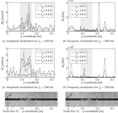
[image:29.595.113.515.246.630.2]

The underlying physical phenomena are still not understood, see section 1.3. However most obvious is a varying stiffness across the damage interface. These asymmetric stiffness effects and energy dissipative mechanisms such as friction, hysteresis and thermo-elastic phenomena can also be possible physical phenomena. When the pump and carrier frequencies are both applied to the previous discussed structure in [3], mostly amplitude modulations are present in the damaged region. The latter can be seen in figure 2.3. Both the clapping and kissing damage behaviors result in mainly amplitude modulations in the damaged area. It can therefore be concluded that the nonlinearity will be of a displacement type. Frequency modulation does also occur in the structure. Since this FM is not concentrated in the damaged region, it can only be used to globally indicate if this specific structure is damaged or not.

Figure 2.3: The (a, c) amplitude and (b, d) frequency modulation distributions of the carrier response for three pump excitation amplitudes. The results forf p= 1455 Hz (clapping mode) are shown in (a, b), while (c, d) show the results forfp= 2340 Hz (kissing mode). The carrier frequency was 50 kHz for all cases. This figure and information is taken from [3].

2.3 Two-tone forced vibration of a nonlinear system

To get a better understanding how the nonlinearities result in a modulated signal, an analytical obtained response of a simplified 1-DOF nonlinear system is discussed by Ooijevaar [3]. These analytical derivations will be discussed and expanded in this section.

(30)

2.3.1 Quadratic displacement nonlinearity

The clapping and kissing behaviors can probably best be approached with a quadratic displace-ment nonlinearity as concluded in [3]. This type of nonlinearity is analytically investigated by Ooijevaar for 1-DOF nonlinear system. There is however no mention how to verify that the ob-tained signal is only modulated in amplitude. The next section will focus on the same derivations in more detail and also provide a quadratic velocity nonlinearity.

A nonlinear multi-DOF system, the first part containing linear terms and the second part con-taining nonlinear terms, can be expressed as:

¨

q+ω_n,2₀q=−f(q,q˙), (2.12)

in which ¨q,q˙ and q are the normalized acceleration, velocity and displacement vectors in one direction. Note that the eigenfrequency ω0 is a scalar. There are however multiple solutions

for the eigenvalue problem; the number of eigenfrequencies n corresponds to the number of independent equations of the system n. A multi-DOF system with a quadratic displacement nonlinearity and two tones forced vibrations can be expressed analytically as:

¨

q+ω2n,0q=−q2+Fpcos(ωpt+φp) +Fccos(ωct+φc) (2.13) When using a perturbation technique based on a power series, the first-order steady state solution

q(t) is expressed as:

qtotal(t) =Ap,ncos(ωpt+φp) +Ac,ncos(ωct+φc)−

2ω2

n,0

(A2_p,n+A2_c,n)

−

2(ω2

n,0−4ωp2)

A2_p,ncos(2ωpt+ 2φp)−

2(ω2

n,0−4ωc2)

A2_c,ncos(2ωct+ 2φc) +Asb1,ncos((ωc−ωp)t+φc−φp) +Asb2,ncos((ωc+ωp)t+φc+φp),

(2.14)

in which:

Asb1,n=

−Ap,nAc,n

ω2

n,0−(ωc−ωp)2

, Ac,n =

Fc

ω2

n,0−ω2c

,

Asb2,n=

−Ap,nAc,n

ω2

n,0−(ωc+ωp)2

, Ap,n=

Fp

ω2

n,0−ωp2

.

When only a narrow band response around the carrier frequency is considered, equation (2.14) can be expressed as:

qbp(t) =Ac,ncos(ωct+φc) +Asb1,ncos((ωc−ωp)t+φc−φp) +Asb2,ncos((ωc+ωp)t+φc+φp),

(2.15)

This is, according to Ooijevaar [3] in the 1-DOF presentation, an amplitude modulated response signal. When equation (2.15) is elaborated the total narrow band response is expressed as:

qtotalbp(t) = n

X

k=1

(Ac,kcos(ωct+φc) +Asb1,kcos((ωc−ωp)t+φc−φp) +Asb2,kcos((ωc+ωp)t+φc+φp)),

(2.16)

where k= 1,2,3....nare the degrees of freedom with nthe total amount of DOF’s. Note that

qtotalbp(t) is a scalar and not a vector anymore. When it is assumed that the terms with a certain frequency (ωp, ωc and the sidebands (ωc±ωp)) will only contribute to the total response when their frequency corresponds with an eigenfrequency of the system (ωp,0, ωc,0 and the sidebands

(ω(c±p),0), the total narrow-band response will become:

qtotalbp(t) =A0_ccos(ωct+φc) +A0sb1cos((ωc−ωp)t+φc−φp) +A0sb2cos((ωc+ωp)t+φc+φp)

(31)

in which:

A0sb1=

−A0_pA0_c ω2

(c−p),0−(ωc−ωp)2

, A0c=

Fc

ω2

c,0−ωc2

,

A0_sb₂= −A 0 pA0c

ω₍2_c₊_p₎_,₀−(ωc+ωp)2

, A0_p= Fp

ω2_p,₀−ω2

p

.

Compared to section 2.1, the narrow-band signal shows differences with an actively modulated signal. The carrier amplitude is in the output signal multiplied by the term:

1 [ω2

c,0]−ω2c

. (2.18)

The amplitude of the sidebands are multiplied by the term:

(ω2_p,₀−ω2_p)(ω2_c,₀−ω2_c) (ω2

(c±p),0−(ωc±ωp)

2₎. (2.19)

From equation (2.18) it can be concluded that the amplitude of the central carrier in the output response is not constant for different carrier frequencies, compared to the active amplitude mod-ulation in section 2.1. From the second statement in equation (2.19) the observations in [19] are proven, certain combinations of the carrier and pump frequency do give the highest signal mod-ulations. Also concluding from equation (2.19) is that the signal modulations will be the highest if for the carrier, pump and sideband frequencies, natural frequencies of the system are chosen as is shown in [29]. The latter can be visualized. The expression for the narrow band response in equation (2.15) is plotted withFp= 8 N,Fc = 1 N,= 0.04,ωp= 2·π·10 rad_s andωc= 2·π·500

rad

s , see figure 2.4. The terms from equation (2.18) and (2.19) give a difference between a natural

frequency of the structure with the carrier frequency and the sideband frequencies. These have to have minimal difference such that the sidebands can be noticed in the frequency spectrum, so a difference of (ω2

c,0−ω2c) = 1

rad s , (ω

2

p,0−ω2p) = 1

rad

s and (ω 2

(c±p),0−(ωc±ωp)

2_{) = 1} rad s is

chosen for figure 2.4. This consequently shows that the carrier frequency should be a lot closer to a natural frequency than the pump frequency due to the quadratic terms.

(32)

[image:32.595.100.475.124.406.2]

Figure 2.4: The bandpass filtered and modulated carrier response of fp = 10 Hz, fc = 500 Hz and e= 0.04 caused by a quadratic displacement nonlinearity.

2.3.2 Quadratic velocity nonlinearity

Not only nonlinearities in terms of displacement could cause the signal modulations in VAM. The dissipative nonlinearities such as hysteresis are most likely caused by a quadratic velocity nonlinearity. This nonlinearity will be investigated in this section with the same method as in section 2.3.1. A multi-DOF system with a quadratic velocity nonlinearity and two tones forced vibrations can be expressed analytically as:

¨

q+ω2_n,₀q=−q˙2+Fpcos(ωpt+φp) +Fccos(ωct+φc) (2.20) The complete derivation can be found in appendix B. When the first order nonlinear solution is considered and when only the frequencies around the carrier signal are taken into account, the following narrow band response is obtained:

qbp(t) =A0ccos(ωct+φc)

−A0_sb₁ωpωccos((ωc−ωp)t+φc−φp)−A0sb2ωpωccos((ωc+ωp)t+φc+φp)

(2.21)

A0_sb₁= −A 0 pA0c

ω2₍_c−p₎_,₀−(ωc−ωp)2

, A0_c = Fc

ω2_c,₀−ω2

c

,

A0_sb₂= −A 0 pA0c

ω2

(c+p),0−(ωc+ωp)2

, A0_p= Fp

ω2

p,0−ωp2

.

(33)

frequency modulation, the extra term ωpωc would mean the difference between AM and FM. When comparing this assumption with equation (2.4) and (2.9), it is however not in line with the obtained expressions for the active controlled AM and FM. The difference between the active AM and FM in equation (2.4) and (2.9) is that the amplitudes of the sidebands are multiplied with _ω1

p and not withωpωc.

The expression in equation (2.21) is plotted in figure 2.5 with again the same values: Fp= 8 N,

Fc = 1 N,= 0.04, ωp= 2·π·10 rad_s , ωc = 2·π·500 rad_s , (ω2c,0−ωc2) = 1

rad s , (ω

2

p,0−ωp2) = 1

rad

s and (ω 2

(c±p),0−(ωc±ωp)2) = 1 rads . The amplitude of the plotted function is considerable

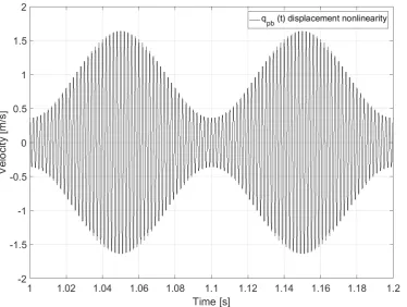
[image:33.595.132.505.270.570.2]

higher than in figure 2.4. This is caused by the multiplication of the amplitudes of the sidebands byωpωc. It is also clear that there is more than 100 % amplitude modulation when figure 2.4 is compared with figure 2.1(b).

Figure 2.5: The bandpass filtered and modulated carrier response of fp = 10 Hz, fc = 500 Hz and e= 0.04 caused by a quadratic velocity nonlinearity.

2.4 Selection of the excitation frequencies for VAM

From the previous section it can be concluded that the excitation frequencies for VAM have to be close to a natural frequency of the investigated structure to give noticeable signal modulations. This has also been concluded in different studies in the literature [3, 29]. The damages in these studies are however not controlled and therefore it is very hard to find a relation between the natural frequencies of a damage(d structure) and the carrier frequency. In this thesis a composite plate with an artificial delamination is considered, such that the global eigenfrequencies of the entire plate and the local eigenfrequencies of the delamination can be determined. Note that the modal density of the global eigenfrequencies will become higher in higher frequency ranges. The selection of the pump frequency seems to be not that difficult for a test specimen. The frequency response functions can be determined for different spatial points in a controlled test

(34)

setup and the accompanied operational deflection shapes can be visualized. A global natural frequency in the lower frequency ranges is selected as pump frequency with a desired operational deflection shape. It should however be stated that the pump frequency selection is more com-plicated when only the pristine global dynamic behavior is known and the (size of the) damage is unknown: the natural frequencies and accompanied operational deflection shapes will differ depending on the damage (size). The global natural frequencies with their operational deflection shapes are first determined numerically for the pristine case. Also the local frequency behavior will be approximated analytically for an artificial delamination. In section 3.3.1, the natural frequencies of the plate will be determined experimentally for the damaged scenario.

2.4.1 The global eigenfrequencies of a composite plate

The global eigenfrequencies of the plate are used in section 3.1.2 to determine the dimensions of the experimental specimens. Limitations on the dimensions and the lay-up are caused by the production method and the measuring equipment, therefore only the numerical model is briefly discussed in this section. The numerical model is created in Ansys Mechanical APDL 14.0, a rectangular composite plate. Shell elements can be assigned with a shell section that contains the number of plies, the ply thickness and the ply orientation. An area-based model with shell elements can be used for a composite plate since the thickness of the plate is relative small compared to the length and width. Another option is creating a model in Ansys based on solid elements. Every ply has to be meshed separately in this case and the material properties have to calculated for every ply since a certain ply orientation has influence on these properties due to the anisotropic properties of a composite ply. However a numerical model based on solid elements is not very suitable for this thin walled structure. It requires a very dense grind in-plane which will result in a lot of elements since a large aspect ratio will give poor results. Moreover there is a high risk of locking since the dominant deformation mode is bending.

(35)

Figure 2.6: The 11th mode of [0/90/45/−45]2, scomposite plate, obtained with Ansys.

2.4.2 The local eigenfrequencies of the delamination

The damaged composite plate with the artificial delamination can be represented as in figure 2.7. When H2 << H, the volume with thickness H2 and radius R will be assumed to show

the clapping behavior [31] and it is therefore assumed that this volume has to be excited by the carrier wave. The volume with thickness H2 and radius R will therefore be treated as a

separate circular plate with specific boundary conditions, this is called ‘the free model theory’. This model has shown to be physically inadmissible [31], the delaminated layers deform freely without touching each other. The ‘constrained theory’ in which the delaminated layers are assumed to kiss each other and are allowed to slide over each other is physically admissible [31]. The local eigenfrequencies will be estimated with the ‘the free model theory’ in this thesis, even though the ‘constrained theory’ model will give more accurate results. The actual local eigenfrequencies are assumed to be in between the eigenfrequencies of a boundary condition of clamped (upper limit) and simply supported (lower limit).

(36)

Figure 2.7: Top and side view of a composite plate with a delamination.

When the thicknessH2, the radiusRof the artificial delamination, the material properties, the

[image:36.595.171.385.102.363.2]

number of layers with their respective thickness and orientation, and the material properties are known, the flexural natural vibrations can be calculated with two different boundary conditions: simply supported and clamped. The different modes are given in figure 2.8 as can be seen in [32].

Figure 2.8: The first 5 modes of simply supported (SS) and a clamped (C) circular plate as in [32]. The modeirefers to the number of circular nodesjof the circular plate and the number of nodal diameters k.

The differential equation describing the circular plate in a polar coordinate system can be ex-pressed as [32]:

∆r∆rWb+ω2

J D(1 +

mD

J S)∆rWb+ω

2m

D( ω2J

S −1)Wb= 0, (2.22)

in which the solution (natural vibrations) can take the form ofWb(r, φ, t) =W(r, φ) sinωt and

Frequency optimisation for damage identification using the Vibro Acoustic Modulation method

Faculty of Engineering Technology

Research group Dynamics Based Maintenance