Filter Bubbles in Opinion Dynamics

F.L.H. K

lein

S

chaarsberg

J

une

24, 2016

Abstract

This paper proposes and analyzes a model of opinion dynamics which produces the behavior of filter bubbles. Filter bubbles are feared to seriously narrow the perspectives of individuals in a society, a consequence of the omnipresent online personalization algorithms. This paper produces a full model development description, based upon fundamental assumptions. It is shown that the model presumably asymptotically converges into one or more clusters of opinions. Furthermore, configurations are described under which the model produces filter bubbles.

key words: opinion dynamics, continuous opinions, cluster formation, filter bubbles

1.

I

ntroduction

The online world as we know it today is highly tailored to our personal interests. Personalization algorithms determine what you see and more importantly what you do not see, all based on information that was gathered about you. These algorithms lead to a so called personalfilter

bubble. This filter bubble is your own personal unique universe of information that you live in

online. More specifically, a filter bubble is the result of a personalized search in which a website algorithm selectively guesses what information its user would like to see, based on information about the user such as location, past click behavior and search history.

“ It will be very hard for people to watch or consume something that has not in some sense been tailored for them”

Eric Schmidt, Google

The name ‘filter bubble’ was coined by Eli Pariser. In a TED talk [1] Pariser makes a plea that we take seriously on the (negative) effects of these personalized filters. The vast amount of information that is currently available on the

web calls for a refined (possibly personalized) selection, which may be found in these selective algorithms. The danger lies in the fact that personalization is now found nearly everywhere on the web. For example, there is no standard Google anymore: for identical search queries, different people might get very different results. Pariser states that the personalization in the Google search engine (without being logged in to a Google-account) is based on 57 input signals. These input signals include anything from the computer that you are using to search history to the time you are spending on certain websites.

It is not only Google that uses personalization, it is nearly every site on the web, including websites that provide our newsfeed. Pariser names ‘The Washington Post’ and ‘The New York Times’ as examples. He states that these personalized filters are moving us very quickly towards a world in which the Internet is showing us a world it thinks we want to see, but not necessarily what we

needto see. What is in your filter bubble depends on who you are and what you do, but you do not decide on what gets in. More importantly, you do not actually see what gets edited out.

In his TED talk Pariser states, in agreement with the author of this paper, that “if algorithms are going to curate the world for us, and they are going to decide what we get to see and what we do not get to see, then we need to make sure that they are not just keyed to relevance. We need to make sure that they also show us things that are uncomfortable, challenging or important, in other words: other points of view”.

With the Internet currently being one of the largest, and maybe the largest sources of news, information and communication, the question arises whether a mathematical model can be made that mimics the effect of the personalization algorithms. For this research, a model is sought in the field ofopinion dynamicsthat can illustrate the effect of personalization algorithms on opinion development. This will help get a better estimate the costs and risks of these algorithms.. To the best knowledge of the author, a model that studies filter bubbles in opinion dynamics has not yet been developed.

The term ‘opinion dynamics’ encompasses a wide class of models that describe the evolution of opinions of individuals1 within a group. Some of these models that will be of use for this paper, are summarized in section 2. In general, in models in opinion dynamics a set of agents is considered where each holds an opinion from a certain opinion space. For continuous opinions this opinion space is typically defined as a certain interval of real numbers. An agent may change his or her opinion when he or she gets aware of the opinion(s) of others in the group.

In this paper a model is proposed that mimics the effect of online personalization algorithms in the field of opinion dynamics, based upon some fundamental assumptions. The goal of this model is to explore the behavior and influences of personalization in opinion dynamics. The resultant model significantly steers and thus modifies the opinions of individuals within a group, thereby creating filter bubbles. Moreover, under certain conditions the model shows how individual opinions may merge into one or more non-communicating clusters of individuals sharing opinions.

This paper is organized as follows: Section 2 gives anoverview of work that is relevant to for this paper. Section 3 reports on the full establishment of the model that is presented. It describes the fundamental assumptions on which the model is based, as well as a step-by-step translation of these assumptions into the model. The behavior and properties of this model are documented in section 4. The overall conclusion of this paper is stated in section 5.

ModelContext andNotation

Opinion dynamics can be put in many contexts. Therefore it is important for the reader to be aware of the context relied on when writing this paper. The establishment of the model, as presented in section 3, is for the largest part based on this context. That is decisions and assumptions that are made, and the goals are set with this context in mind.

The context for which the model is developed is an online social network. Typical examples are Facebook and Twitter, but one can also include any online forum, or anything similar. What characterizes this context is that people in the network (the users) do not meet in person, but instead read each other’s posts. The influence on opinions is therefore one-way, that is the ‘poster’ influences the opinion of the ‘reader’ (and not vice versa). For generalizing such context, the notation as described here is relied on throughout this paper.

A social network is represented by a directed graphG. This graph consists of p≥0 nodes which represents the people (or users) in the network. LetP denote the set of persons in the network such that|P |= p, where|P |denotes the cardinality ofP. Also, letCdenote the set of network

connections(the direct connection between two people), that is the set of edges ofC. Therefore,

in shortG can be written as G = (P,C). Let G be such that(i,i) ∈ C/ for all nodes i, so G is loop-free. For each nodei∈ P the group of friends (or connections) of individualiis denoted by Fi ={j∈ P:(i,j)∈ C}. For this nodei∈ P the degree of this node (the number of ‘friends’ ofi) is equal to|Fi|.

The opinion or belief of an individual is denoted by a real number between 0 and 100. At timek

(k=0, 1, 2, ...) the opinion-state of individualiis denoted asxi(k)∈[0, 100]. The opinion state of all individuals in the network is represented by avector of beliefs,x(k)∈Rp_{. The vector of initial} opinions is denoted asx(0).

2.

L

iterature

R

eview

This section gives an overview of relevant work on opinion dynamics that has been done up to now. It presents a general overview, as well as a more detailed description of some fundamental models.

Models that would nowadays be regarded as opinion dynamics date back to papers by French [2], Harary [3] and DeGroot [4]. In these models opinion updates occur according to a linear, and often convex combination of an individual’s current opinion, the opinions of others, and possibly the agent’s initial opinion.

For this research only models of continuous opinions are considered. Multiple models on binary opinions have been studied though, for example in [5] and [6]. Notable models in continuous opinion dynamics include models based on bounded confidence, for example models by Deffuant et al. [7] and the Hegselman and Krause model [8], and models that include prejudices where an individual’s initial opinion is also taken into account, for instance the model by Friedkin and Johnson [9]. Throughout the years, these models have been extensively studied and extended. One extension one might encounter is that of asynchronous opinion updates, for instance by Frasca et al. [10]. Other studies on for example model convergence are presented in [11], [12] or [13].

The remainder of this section is devoted to briefly summarizing models based on bounded confidence, and a more detailed summary of the model by Friedkin and Johnson [9], and the Friedkin Johnson model with asynchronous updates presented by Frasca et al. [10].

2.1. Models of bounded confidence

shall only update its opinion with another’s if their opinion difference is less than a certain confidence bound denoted bye. The Hegselmann-Krause model yields to a synchronous opinion

update, whereas the Deffuant-Weisbuch model uses pairwise encounters (asynchronous). These models with bounded confidence typically restrict an individual’s view to only certain other individuals, for whom the absolute opinion difference is less than a certain confidence boundei.

For example for the Deffuant-Weisbuch an opinion update typically looks as follows:

xi(k+1) =

(_xj(k)+xi(k)

2 if

x_i−x_j(k) ≤e_i,

xi(k) otherwise.

(1)

Figure 2.1 shows a typical simulation of a model of bounded confidence. In figure 2.1, time steps are set out on the horizontal axis, whereas the vertical axis denotes the opinion values (in this case these lie in the interval[0, 1]). Since models of bounded confidence will not be further considered

Figure 2.1: Simulation of a model of bounded confidence. Left: confidence bounde=0.15, right: e=0.25. [8]

in this paper, the information given above should be sufficient for the reader to get the main idea of these models. For more information the reader is suggested to consult [7] and [8].

2.2. Friedkin andJohnson’s model

The model presented in [9] is defined as follows: LetW ∈Rp×p_{be a (nonnegative) row-stochastic} matrix, theweight matrix. The elementswij denote the weight individualigives to the opinion of individualjin the network. We letwij =0 if there is no direct connection betweeniandj, i.e.

(i,j)∈ C/ . LetΛ∈Rp×p_{be a diagonal matrix which describes thesensitivityof each individual} to other’s opinion. This matrix Λis defined asΛ = I−diag(W), where diag(W)denotes the diagonal matrix containing the corresponding diagonal elements ofW.

In this model, thesynchronousdynamics of opinions is given by:

x(k+1) =ΛWx(k) + (I−Λ)x(0). (2)

In (2) the individual’s opinion at time stepk is (always) influenced by the individual’s initial opinion x(0), this aspect is sometimes referred to asprejudices. Note that these prejudices are eliminated ofΛ=Iis set. The opinion profile at time stepkmay be written to be equal to:

x(k) = (ΛW)k+

k−1

∑

(ΛW)i(I−Λ)

!

It has been proven in [10] that the limit behavior of the opinions can be described as follows: Assume that from any nodel∈ P there exists a path fromlto a nodemsuch thatWlm>0, then the opinions converge and

x∞:= lim

k→+∞x(k) = (I−ΛW)

−1_{(I−Λ)x(0).}

In their 2013 paper [10], Frasca et al. extended Friedkin and Johnsen’s model to an asynchronous model where agents (asynchronously) interact in pairs, in this paper this model is referred to as the ‘Frasca Model’. These pairs are chosen according to a random process, and the ‘interaction in pairs’ is referred to asgossiping. A model that includes asynchronous opinion updates better fits the behavior of individuals in a social network, since they typically read one post at a time, and therefore they may update their opinion at every read.

The Frasca Model [10] is described as follows: Each agent i ∈ P starts with an initial belief

xi(0) ∈ R. At each time ka directed link is randomly sampled from the social network, i.e. randomly sampled from a uniform distribution overC. If link(i,j)is selected at timek, then agent

iupdates its opinion to a convex combination of its previous opinion, the opinion of j and its initial opinionxi(0). The update takes place according to (3).

xi(k+1) =hi (1−γij)xi(k) +γijxj(k)

+ (1−hi)xi(0),

xl(k+1) =xl(k)∀l∈ P \ {i}.

(3)

Here the coefficientshiare the diagonal elements of the diagonal matrixH∈Rp×p, andγijare the elements of matrixΓ∈Rp×p_{. These matrices are determined as follows:}

FirstlyD∈Rp×p_{is defined to be the degree matrix ofG, i.e. a diagonal matrix where the diagonal} entriesdiare equal to the degreedi=|Pi|. In social network terms, one could state thatdiequals the number of friends of individuali.

Then

hi = (

(di−(1−λii))/di ifdi 6=1,

0 otherwise.

γij=

     

    

di(1−hi)+hi−(1−λiiwii)

hi ifi=j,di6=1,

λiiwij

hi ifi6= j,di 6=1,

1 ifi=j,di=1, 0 ifi6= j,di =1.

(4)

3.

M

ethods

In this section a model is presented here that shows how filter bubbles of opinions may form across a social network. In the remainder of this paper, this model is referred to as thefiltered model. In section 4 the results of the filtered model will be compared to the Frasca Model [10]. The eventual goal of this filtered model is to personalize the communication of the individuals in the network, and thereby deliberately steer opinions in certain personalized directions and eventually create filter bubbles.

The general structure of this section is as follows: Firstly, the fundamental model assumptions that form a foundation for the filtered model are presented. Secondly, this foundation shall be translated into a mathematical framework, that is, a rough outline for the model is presented. The main bodywork of this section, paragraph 3.2, is formed by the actual establishment of the filtered model. This section is concluded with a summary which recapitulates the full model, see paragraph 3.3.

Recall that in the asynchronous model presented by Frasca et al. [10] an agent couple(i,j), that is an edge fromG, is selected uniformly overC. For the filtered model this asynchronous opinion update is adopted, since the author believes that this model sufficiently represents communications within an online network. The main feature of this model is an adapted procedure for selecting these edges. That is, edges will not be selected uniformly overC, but will be drawn from a yet to be determined probability distribution. In this probability distributionPk(i,j)denotes the probability of sampling (directed) edge(i,j) at timek. This adapted sampling method shall replicate the personalized feature of the filtered model. For the filtered model, opinions are updated according to equations 3 and 4. Prejudices are not included though, that isΛ=I.

Assumption 1 and 2 below formulate the fundamental assumptions of the filtered model. Both assumptions are based upon common underlying principles of current online filtering algorithms [14].

Assumption 1. People with alike opinions are more likely to be interested in each others posts.

This assumption is related to the goal of the filtered model in the following way: Given a certain individualiin the network, the goal is to filter out posts of other people that have a very different opinion. In terms of sampling, the probability of sampling people with alike opinions shall be (considerably) larger than people with different opinions.

Assumption 2. People that are interested in each others opinion are more likely to read each others posts, they might even search for them. In terms of edge sampling: the more times edge(i,j)has been sampled, the more likely it is to be re-sampled.

Relating assumption 2 to the model’s goal as well, one can say that this assumption relates to the viewing history, that is, the sampling history. Again, the probability of sampling people with a rich history shall be (considerably) larger than people with little sampling history.

In the same context, assumption 4 indicates that the number of posts a user reads and/or posts is equal for all users, given a certain time span.

Assumption 3. The network graphGis complete.

Assumption 4. All agents in the network are equally active in the network.

Assumption 4 relates directly to the procedure for edge selection for simulations. By assumption 4 the procedure for selecting edges fromCmay be defined as follows:

Definition 1(Sampling procedure). Selecting edges fromCat timekis conducted according to the following two steps:

(i) The first individual, denoted by N1, will be drawn uniformly from P. That is,

Pk_{(i) =} 1 p.

(ii) The second individual, denoted byN2, will be drawn fromPk(i,j|i).

In this way the probability of sampling edge(i,j)at timekis denoted byPk(i,j) =Pk(i)Pk(i,j|i).

In the remainder of this section the focus reduces to finding an expression forPk_{(i,j|i). This} expression will be based on assumptions 1 and 2. Paragraph 3.1 presents a mathematisation of the model assumptions that were presented in this section, as well as a rough outline of the model.

3.1. Model outline

Assumptions 1 and 2 in the previous section translate the two main parameters of the filtered model. Namely, the probability distributionPk(i,j|i)will depend on(absolute) difference in opinion

and thesampling history. The following two definitions formally define these parameters. Definition 2 follows directly from assumption 1, whereas definition 3 follows from assumption 2.

Definition 2. Let N1=ibe fixed. The absolute difference in opinion between agentiand (other) agentsj∈ Pat timekis defined as∆k_ij:=|xi(k)−xj(k)|.

Definition 3. The matrix C(k) ∈ N₀p×p is defined to keep track of the sampling history up until timek. The elements ofC(k), denoted by,c_ijk ∈N0, indicate the number of times (directed) edge(i,j)has been sampled.

A general expression forPk(i,j|i)in terms of∆k_ijandck_ijis presented in (5). This equation states thatPk(i,j|i)is proportional to some function f(∆k_ij,ck_ij), an explicit expression for which is yet to be determined. For the sake of avoiding unnecessary complexities, the author deliberately chooses to separate the influences of∆k_ij andck_ijinto some functionsg(∆k_ij)andh(ck_ij). These functions are ‘combined’ by some operator ‘?’. Note also thatαandβare scaling factors forgandhrespectively,

andβare both nonnegative in any case.

Pk_{(i,j|i)∝ f(∆}k

ij,ckij) =αg(∆ijk)?βh(ckij). (5)

For finding an explicit expression for f(∆k

ij,ckij)in (5), a list of requirements will be set up. Most of these requirements follow from the assumptions made in the previous section.

List of requirements:

(i) Making sure that sampling individuals with alike opinion is favored over individuals with a different opinion requires that f is descending in∆k_ij, meaning ∂f

∂∆<0. To amplify this effect,

the following requirement is set as well: ∂2g

∂∆2 >0.

(ii) Also, individuals with a rich sample history are favored over those with little. Therefore the requirements that follows is: f is increasing inc, meaning ∂_∂cf >0.

(iii) To prevent problems in scaling f to a probability mass function later on, the following requirements follow for g and h: Firstly, g(∆k_ij) > 0 for all∆k_ij ≥ 0 (note that ∆k_ij ≥ 0 is satisfied by the definition of∆k_ij). Secondlyh(c)>0,∀c≥0, in particular forc=0. One may seth(0) =ξ, for certainξ>0.

(iv) In combining the influences of g andh in (5), it has to be made sure that the range of g

matches that ofh(and vice versa).

(v) The influence of sampling history onPk(i,j|i)may not be too high if hardly any history has been built up yet.

Implementing these requirements into an expression for the different elements of (5) is described in paragraph 3.2. The reader could decide on leaping to section 3.3, where the finalized model is presented.

3.2. Model establishment

The following paragraphs describe a step-by-step translation of the requirements presented in the previous section into an explicit expression for (5).

3.2.1. Difference in opinion

The requirements described in paragraph 3.1 lead to a function corresponding to the sketch in figure 3.1. A function that describes the required sketch is of the formg(∆k_ij) = 1

p(∆k

ij)

, for some

functionp(∆k_ij).

For the actual choice ofg(∆k_ij) = 1

p(∆k

ij)

it is wise to first examine the domain ofg(∆k_ij). As opinions

are represented by a real number in the interval[0, 100], we have that also∆k_ij ∈[0, 100], which is the domain ofg(∆k

ij). Therefore it has to be made sure that admissible∆kij should yield that

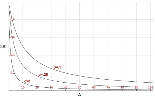
Figure 3.1: Three plots of functions forg(∆k_ij), different levels of sensitivity.

For the range ofg(∆k_ij)it is desired that it is bounded, as to fit the range ofh(c)to it later on. The range ifg(∆k_ij)is therefore set to[γ, 1], where 0<γ<1,g(0) =1, andg(100) =γ.

A function that fulfills all requirements is the following:

g(∆k_ij) = 1

σ∆k_ij+1 , where

σis a measure for the vigor of descent. (6)

Suitable choices forσareσW =0.1 for weak,σM=0.25 for mediocre, andσV =1 for vigorous descend. Please see figure 3.1 for the plots ofg(∆k_ij)for these values ofσ. In section 4 the influence

of this parameterσon the model behavior will be examined.

3.2.2. Sample counter

For the range ofhto match that ofg, it is set to the interval(0, 1). The function of the following form fits all the requirements:

h(ck_ij) = c

k ij

c_ijk_,max+1 !2

, where ck_ij,max :=max j|i {c

k

ij}. (7)

Note though that the range ofh is typically equal to 0,h(cij,max)

. It is worth noticing that the upper bound of this interval quickly approaches 1 asck

ij,maxincreases.

3.2.3. Other parameters

The influences of (6) and (7) depend on the choice ofαandβin (5) respectively. The influence of

opinion difference, i.e. α, may be chosen equal over time. Thereforeαis set equal to 1. When it

comes to the choice ofβ, more caution is required.

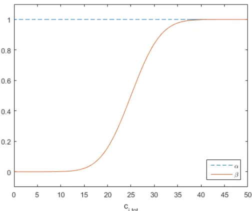
Basically,βdetermines the influence of ‘history’ on the edge sampling. Therefore it is not desired

requirement is set that 0 ≤ β α = 1 when c_ik_,tot := ∑j|ic

k

ij is still low. Then, as soon as

ck_i,tot increases, also β increases asymptotically toα = 1. This desired behavior ofα and βis

demonstrated in figure 3.2.

Figure 3.2: Behavior ofαandβ.

The relation of β to ck_i,tot can be described by a function of the same form as the cumulative

distribution function of a normal distribution, i.e. a function of the form

β(ck_i,tot) =

1 2

"

1+erf c k

i,tot−p1

p2 √

2 !#

. (8)

Where parametersp1andp2determine the location of the inflection point and the steepness of the function, respectively. If these parameters are chosen asp1=25 and p2=10, then the plot in figure 3.2 is acquired. Therefore we determine the value ofβas follows:

βk_i :=β(ck_i,tot) =

1 2

"

1+erf c k

i,tot−25

10√2 !#

. (9)

It is assumed here that enough ‘history’ has been build up after approximately 20 samplings, that is whenβk_i starts increasing to 1 (see figure 3.2).

3.2.4. Intermediate recapitulation

The previous paragraphs have led to an expression for f(∆k_ij,ck_ij)in (5). The final expression of

f(∆k

ij,ckij)is given below for the benefit of clarity.

f(∆k_ij,ck_ij) =αg(∆k_ij) +βh(c_ijk) = 1

σ∆k_ij+1

+βk_i

ck ij

ck

ij,max+1

!2

, in which (10)

(i) σis a measure for the intensity, see figure 3.1. Initial choiceσ=0.5;

(ii) βk_i =β(ck_i,tot) =

1 2

1+erf

c_ik_,tot−25

10√2

, andck_i,tot =∑j|icij;

(iii) ck_ij,max=maxj|i{ckij}.

3.3. Finalizing the model

In this paragraph the final expression forPk(i,j|i)is presented. Before that, one final assumption is made.

Assumption 5. The attention and view of an individual is limited to a certain number of people, where this number is denoted byn. Especially in large networks, individuals are assumed to only read a certain portion of new posts instead of all new posts. Besides, the model is asked to make a specific selection of the vast amount of information.

Assumption 5 leads to an important aspect of the filtered model, starting with the following definition:

Definition 4. Letibe fixed and letτbe a positive integer, such thatτ< p. At timekdefine

T_ik(τ):={j1,j2, ...,jτ|1≤n≤τ: jn∈ Fi},

such that f(∆k_ij,ck_ij)≥ f(∆k_il,ck_il)for allj∈ Tk

i (τ)andl∈ T/ ik(τ).

In definition 4,Tk

i (τ)is defined as the collection ofτindividuals for which the value of f is the highest. Recall thati∈ F/ _i. Now define

˜

f(∆k_ij,ck_ij):=

(

f(∆k_ij,ck_ij) if j∈ Tk i (τ), 0 if j∈ T/ k

i (τ),

Pk_(i,j|i):= f˜(∆ k ij,ckij) ∑m|i f˜(∆imk ,cimk )

,

(11)

∑j|iPk(i,j|i) =1. Moreover one finds that

∑

i

∑

Pk_(N

1=i,N2=j) =

∑

i

∑

Pk_(N

1=i)Pk(N2=j|N1=i)

=

∑

i

Pk_(N

1=i)

∑

Pk_(N

2=j|N1=i) =1.

4.

R

esults

In this section the characteristics and the properties of the filtered model, as is presented in section 3, are described. It contains statements on the behavior of the model one would typically see in simulations, as well as an examination of the influences of the different components of (10). Based upon observations of the model behavior several definitions and claims are stated. This section is concluded with a statistical analysis which states under which conditions the presented filtered model actually alters the opinions of individuals within a group, and when the model leads to the creation of filter bubbles.

4.1. Model behavior

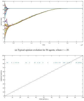
A description of the general behavior of the model is given with reference to a typical simulation result. Figure 4.1a shows such a result. Included as well is a plot which displays the individual’s initial opinion versus its opinion at the end of simulation, see figure 4.1b. An additional simulation outcome is included in appendix B. Figure 4.1 shows the result of a simulation where the number of agents in the network equals 50, andτequals 8. Figure B.1 shows the result of a simulation

whereτequals 25.

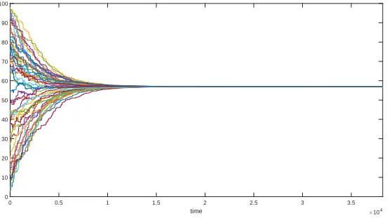
Figure 4.2 shows a typical plot for the model with uniform sampling, as presented in [10], this figure is included for the reader to serve as comparison for the results of the filtered model. As has been proven in [10], this model with uniform sampling always converges to group consensus.

What is typically observed in the simulation results of the filtered model is that individual opinions after some time merge into a subgroup of opinions, a so called cluster (formal definition follows later in this section). Also, it seems that all individuals reach such a subgroup eventually, which will also be proven later on in this section. The number of these subgroups depends on the run, but also depends on the choice ofτ, as will be shown later on. In cases where a simulation leads

to a consensus, as in figure B.1a, its limit value may very well be different than that of the model with uniform sampling. This is illustrated when the reader compares figure B.1a to figure 4.2.

This paragraph is concluded with some formal definitions concerning clusters which will be used to further analyze the model behavior.

Definition 5(Cluster). The set of individualsΩ := {i1, ...,iω}form a cluster at timekif xi = xj holds for all i,j ∈ Ω and also xi =6 xl holds for all i,j ∈ Ω and for all l ∈/ Ω. Moreover the size of the cluster is denoted by|Ω|=ω, that is the number of individuals in

0 1 2 3 4 5 6 7

time ×104

0 10 20 30 40 50 60 70 80 90 100

opinion state

(a) Typical opinion evolution for 50 agents, whereτ=8.

0 10 20 30 40 50 60 70 80 90 100

initial opinions u 0

10 20 30 40 50 60 70 80 90 100

stabilized opinions

(b) Initial versus final opinions for 50 agents, whereτ=8.

Figure 4.1

Definition 6(Stable cluster). The set of individualsΩ:={i1, ...,iω}form a stable cluster if

all of the following properties hold for alli,j∈Ωand for alll∈/Ω:

• limk→∞|xi(k+1)−xi(k)|=0,

• limk→∞|xi(k)−xj(k)|=0, and

• limk→∞|xi(k)−xl(k)|>0.

4.1.1. Model components

In this paragraph the influences of the different components of the model are briefly described. That is, the influences ofg(∆k

0 0.5 1 1.5 2 2.5 3 3.5

time ×104

0 10 20 30 40 50 60 70 80 90 100

opinion state

Figure 4.2: Typical opinion evolution in the Frasca Model.

When only regarding the influence ofg(∆k

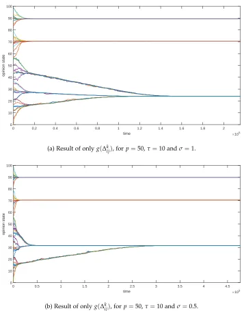
ij), the result is like that of existing bounded confidence models, see figures C.2a and C.2b. A trend that one typically perceives is that different groups of opinions move towards each other slower asσis increased. Though, due to the random behavior

of the model, the simulation time may differ considerably per run. Relating this last finding to figure 3.1, one could say for σ = 1 and fixing individual i, that i is hardly driven toward

individualsjfor which∆k

ij>10. Whereas this is far more likely forσ=0.25. Thereforeσis kept equal to the initial choice of 0.5.

The influence ofh(ck_ij)only is shown in figure C.3. Also,h(ck_ij)alone leads to the formation of clusters. What is typical here is that the lines of opinion evolution are far less separated in groups in the early stage of simulation. In figures C.2a to C.2b this separation is far more obvious.

Lastly, ifβis set to 1 for all individuals and all timek, a convergent development of opinions is

still observed. What is typical for these simulations is that some individuals remain ‘in doubt’ on which cluster to choose, this can be observed in figure C.4. This ‘doubt’ for some individuals may be caused by basing the initial sampling on sampling history that is not there, as described earlier.

Overall, one could conclude that the clustering of opinions is caused byg(∆_ijk)as well ash(ck_ij), where both components amplify each other. Besides, the choice of includingβk_i (see (9)) pushes

‘doubtful individuals’ in a certain direction faster.

4.2. Formation of clusters

Experimental results, as were referred to in the previous section, lead to a set of claims, pre-sumptions and statements on the behavior model. This section is devoted to stating and proving, confirming or motivating these claims, presumptions and statements. One can make a rough distinction between claims on convergence, and claims on the manipulation of opinions.

Proof. LetΩ= {i1, ...,iω}form a stable cluster at some timek0, but letω <τ+1. Then for all

i∈ Ωthere exists anl∈/ Ωsuch thatPk(i,l|i)>0. Therefore the probability of sampling edge

(i,l)at some timek>k0is equal to 1.

Then if an edge(i,l)is selected at timek, the opinionxi(k)is updated withxl(k). Given thatxi 6=xl and assuming thatW(i,l)>0, we find thatxi(k)6=xi(k+1). Thereforexi(k+1)6=xj(k+1), for allj∈Ω. So at timek+1 individualihas leftΩ, and thereforeΩis not a stable cluster.

Claim 1 states the relation that a stable cluster implies that it contains at leastτ+1 individuals.

This statement gives rise to a question whether the opposite statement also holds. This opposite claim, including an additional condition, may be found in claim 2 below.

Claim 2. IfΩ={i1, ...,iω},ω>τ, form a cluster at some time k0, and ck_ij0 >c_ilk0 for all i,j∈Ω

and all l∈/Ω, then the individuals inΩconverge to a stable cluster.

Proof. LetΩ={i1, ...,iω},ω>τform a cluster at timek0. Also letck_ij0 >c_ilk0 for alli,j∈Ωand all

l∈/Ω.

It follows that f(∆k0 ij,c

k0

ij)> f(∆ k0 il,c

k0

il), and thereforePk0(i,j|i)>Pk0(i,l|i)holds for alli,j∈ Ω and all l ∈/ Ω. Sinceω > τ, it holds thatPk0(i,l|i) = 0 for everyi ∈ Ω andl ∈/ Ω. Moreover, Pk_{(i,l|i) =0 holds for anyk>k}

0.

It follows thatΩmeets the properties in definition 6, and therefore the individuals inΩconverge to a stable cluster.

More experimental results suggest further claims on the convergence of opinions can be made. For any simulations, convergence is supposed satisfied as soon as the following criterion is satisfied:

kx(k)−x(k−1000)k<10−5. (12)

Note that by the asynchronous opinion update, a criterion such askx(k)−x(k−1)k<10−5does not suffice.

All 4900 simulations for appendix D show such a convergent simulation result in finite time.That is, all opinionsxi(k)converge to a cluster asktends to infinity. By the means of asynchronous opinion update (3), one finds that this convergence is asymptotic. The following claim proposes a statement on convergence.

Definition 7(Almost sure convergence). x(k)∈Rp_{is convergent a.s. tox(∞)if}

P(limk→∞x(k) =x(∞)) =1.

Presumption 1. The filtered model almost sure converges to some x(∞).

It is presumed that the filtered model converges almost surely based upon the results of a large amount simulations. As stated before, 4900 simulations forp=50 and for different values ofτ

Motivation for the verity of presumption 1 may be sought in papers by Zhang and Hong [15] and another paper by Zhang [16]. These papers analyze convergence and specifically clusterization for an asymmetric variant of the Deffuant-Weisbuch model (bounded confidence). The model presented in these papers uses an opinion update protocol identical to that used in the filtered model, that is equation (3) forΛ=I. The almost sure convergence of such a model of bounded confidence is proven in these papers.

It is believed that the convergence properties presented in [15] and [16] also hold for the filtered model. Reason for this belief is that the filtered model behaves similar to a bounded confidence model, especially at the start of simulation due to the choice ofβk_i (9). Once again, this believe is

confirmed by the simulations, though a formal proof remains a subject for future work.

For the claims that follow, it is assumed that the model converges almost surely.

4.2.1. Number of clusters

Claim 1 implies an upper bound for the number of stable clusters that may emerge, which is b_τ+1p c. Though, except for the trivial result whereb_τ+1p c=1, a result whereb_τ+1p cstable clusters emerge, is hardly ever observed. Moreover, it is often observed that the number of stable clusters that emerge is more or less equal to 1₂bp_τc. This observation on the model behavior leads to the following claim.

Claim 3. On average, a number of stable clusters less than or equal to 1₂b_τpcis observed.

This claim is confirmed by running multiple simulations. That is, for each τ ∈ [1, 49], 100

simulations were run until the convergence property was met (12). Among other data, information about the emergence of clusters was stored. Table E.1 in appendix E shows the outcome of these simulations. The table entries represent intensities on the number of clusters that appeared,that is , for instance forτ =5 a result of 4 stable clusters was observed 30 times. Besides, columns

4 to 6 of table D.1 in appendix D show the average number of clusters, the standard deviation in the number of clusters that emerged, and the highest number of clusters that were observed respectively.

Clearly, the results of the simulations confirm the statement in claim 3. That is, for any value ofτ

the average number of stable clusters that emerged was less than or equal to1₂b_τpc. One could note that the number of clusters that may emerge for smallτis rather broad, therefore no meaningful

statements can be made on this. For larger values ofτone could make a clearer statement on the

number of clusters that might emerge.

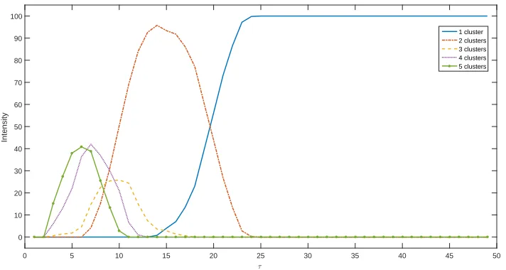
Figure 4.3 shows plots for the number of clusters that emerged in the simulations. Each line represents a certain number of clusters, see the legend. Values ofτare presented on the horizontal

axis, and emergence intensities are shown on the vertical axis. For clarification, forτ = 20 all

0 5 10 15 20 25 30 35 40 45 50

τ

0 10 20 30 40 50 60 70 80 90 100

Intensity

1 cluster 2 clusters 3 clusters 4 clusters 5 clusters

Figure 4.3: Statistics of the number of emerged clusters.

For the figure in which the plots of all emerged number of clusters is displayed, can be found in appendix F. In figure F.1, possibly combined with table E.1, one clearly observes that the spectrum of number of clusters that may emerge forτ<8 is broad. That is, forp=50 one may observe any

of the emerged cluster numbers greater than 2. Whereas, forτ=20 the number of clusters that

will emerge is easier to predict, either 1 or 2.

It is also true that under certain conditions the filtered model produces multiple clusters, and under other conditions only one cluster. This result will be examined in section 4.4. A clear question that arises now is whether the converged opinions in the filtered model are significantly different from those in the model with uniform sampling, and possibly under which conditions. The following paragraph is devoted to answering this question.

4.3. Modification of opinions

Before any statement on opinion modificative properties of the filtered model can be made, a definition of ‘significant difference in opinion’ shall be stated.

Definition 8. Two opinionsxandyare defined as being different if|x−y|>e. Hereeis

defined as being equal to 10% of the length of the total opinion interval. For opinions in the interval[0, 100]it follows thate=10.

Definition 9. Letx(∞)andy(∞)be the converged outcomes of two models on the same social network. Outcomesx(∞)andy(∞)are defined as being significantly different if on average, the individual opinions are significantly different. That is when ∑i∈P|xi(∞)−yi(∞)|

p >

e, for the sameeas in definition 8.

Claim 4. The resultant opinion vector x(∞)of the filtered model is significantly different from that of the uniformly-sampled model.

Claim 4 has been proven/confirmed by executing the Wilcoxon Signed-rank test usingmatlab, for each value ofτbetween 1 and 49. For each of the tests the number of agents was fixed as

p=50, the initial opinionsx(0)as well as the weight matrixWwere randomly generated before the simulations and kept fixed for all runs. Besides, the order in which all the ‘first individuals’ are selected, was randomly determined before the simulations, and these as well were kept fixed for all runs. The testing procedure took place as follows:

For eachτ∈[1, 49], 100 simulations were ran (for a sufficient number of time steps to satisfy 12).

For every simulation the average opinion difference of the group (definition 9) was calculated. For everyτthe Wilcoxon Signed-rank test tests whether the result differs more than 10 or not. The

following Wilcoxon Signed-rank test was performed bymatlab:

H0: ∑i∈P

|xi(∞)−yi(∞)|

p ≤10, the average difference is not significant.

H1: ∑i∈P

|xi(∞)−yi(∞)|

p >10, the average difference is indeed significant.

Thematlaboutput is as follows: h =1 indicates a rejection of the null hypothesis, andh= 0 indicates a failure to reject the null hypothesis at the 5% significance level. The outcome of the tests presented in columns 2 and 3 in table D.1 in appendix D.

The statistics show a clear confirmation of claim 4. That is, the filtered model results in a significant change in group opinion, wheneverτis chosen smaller or equal to 33. From these results one can

also conclude that forτ>33 all individual opinions converge to the same limit, where this limit

is not significantly different from the opinion limit in the model with uniform sampling.

The previously shown statistical tests were preformed for a fixed number of group size, that is for

p=50. One might ask how the model behaves for larger group sizes, for example for p=100,

p=200 or any otherp>50. Based upon experimenting with the group sizes, the following claim is made.

Presumption 2. Upscaling p andτ(by the same scale) does not change the outcome of the model.

This presumption states that the result (number of stable clusters) for p=50 andτ=10 is the

same as forp=100 andτ=20. We may reasonably assume that this is the case, for the values

4.4. Relating results to filter bubbles

Up until now any relation to filter bubbles has been omitted. In this section the results from the previous sections are related to filter bubbles. The processes that lead to the creation of filter bubbles have several consequences. The consequences that are considered in this section are ‘creation of noninteracting subgroups’, ‘changing opinions’ and ‘personal filter bubble’.

One property of the filter bubble is that it deliberately changes the opinions of people. In section 4.3 it has been shown that the filtered model does exactly this forτ ≤33, see table D.1. Even

though this steering effect on opinions is a key aspect of filter bubbles, in this model it does not imply that individuals have been split up in several groups of different opinions.

This last phenomenon may be observed for τ ≤22, again see table D.1. If the model leads to

the formation of stable clusters, then these are non-communicating. This means that each cluster forms an isolated group, one could call this group a ‘bubble’. Due to the design of the filtered model, in such a bubble people only get to communicate with others that have alike opinions.

As described in the Introduction of this paper, Eli Pariser defines the filter bubble as a personal thing. That is, the bubble is seen from the point of view of an individual, and not as a birds-eye view upon a group. The following definition describes apersonalfilter bubble, as Pariser describes it.

Definition 10(Personal filter bubble). The personal filter bubble of individualiis formed by a fixed set of individualsBi(τ) := {j1,j2, ...,jτ|1≤ n ≤ τ : jn ∈ Fi}, such that only posts from individuals from this set are shown.

The following claim (and its proof) states the relation between the filtered model and the emergence of personal filter bubbles.

Claim 5. Any individual i in a stable cluster develops a fixed set of individualsBi(τ)for which

for some k >K (K ∈N) it holds thatPk(i,j|i) 6=0for all j∈ Bi(τ), andPk(i,l|i) =0for all

l∈ B/ i(τ).

Proof. For an individualito converge to a stable cluster, its probability of sampling an individual from that cluster should converge to 1. Therefore individualionly samples individuals from that cluster. For alljin that cluster∆k_ijis equal, therefore the sampling probability depends only onck_ij.

Given a timeK, there exists a set of individualsB_i(τ):={j1,j2, ...,jτ|1≤n≤τ: jn∈ Fi}, such thatcK_ij >cK_il holds for allj ∈ B_i andl∈ B/ _i. ThereforePK(i,j|i)>PK(i,l|i) =0. For anyk≥K

only individuals fromBi are sampled, and thereforePk(i,j|i)>Pk(i,l|i) =0 holds for anyk≥K. HenceB_iforms a fixed set.

4.5. Summary of results

The overall results suggest that the model that was proposed in section 3 leads to the creation of filter bubbles. Under certain model settings (referring to τ) the filtered model leads to a

the model may lead to the clusterization of opinions into non-communicating or isolated groups of individuals. Moreover, the developed model leads to the generation of personal filter bubbles, where a fixed group of individuals form the entire feed for a certain person.

Furthermore, the model has been proven to asymptotically converge to a stable opinion profile. Multiple claims were also made and proven on the number of clusters that may emerge.

5.

C

onclusion

In this paper a model was presented that produces the behavior of filter bubbles in opinion dynamics. This model was built upon fundamental assumptions, based on the principles of current online personalization algorithms. The model was shown to presumably converge into stable clusters of opinions. Besides, the model has also been proven to create personal filter bubbles for each of the individuals in the social network. Furthermore, some interesting claims and statements were made on the model’s properties.

The full filtered model was based on assumptions 1 and 2, together with the requirements presented in section 3.1. Even though these assumptions and requirements are fundamental, the implementation is not unambiguous. In this research a model was established for it that did the job. No research was done to other implementations of these assumptions and requirements. This may be a point for further research. Besides, the current model only contains two main inputs. As briefly mentioned in the introductory section, Google’s personalization algorithms use 57 input signals. Further research may be focused on extending the number of input signals for the model. Lastly, in the current model all sampling history is considered for sampling new edges. One could reasonably assume that more recent history is of more value, than history from longer ago. This feature of weighting or deleting history has not been included, and also this might be a feature for future models.

6.

A

cknowledgements

My most sincere thanks go to my mentor, Dr. Paolo Frasca. I thank him for his useful advice, fruitful discussions and his overall supervision throughout this project. Besides, I thank him for introducing me to the field of opinion dynamics, and that of filter bubbles. I also wish to thank Dr. Miles Macleod and fellow students David Doppenberg and Mike Wendels for their valuable comments and suggestions for the improvement of this work. I wish to thank fellow student Sander Dijkstra for his general additions to this work.

R

eferences

[1] Pariser, Eli:Beware online “filter bubbles”. 2011. https://www.ted.com/talks/eli_pariser_

beware_online_filter_bubbles.

[2] French Jr, John RP:A formal theory of social power. Psychological review, 63(3):181, 1956.

[4] DeGroot, Morris H:Reaching a consensus. Journal of the American Statistical Association, 69(345):118–121, 1974.

[5] Arthur, W Brian:Increasing returns and path dependence in the economy. University of Michigan Press, 1994.

[6] Föllmer, Hans: Random economies with many interacting agents. Journal of mathematical economics, 1(1):51–62, 1974.

[7] Deffuant, Guillaume, David Neau, Frederic Amblard, and Gérard Weisbuch:Mixing beliefs

among interacting agents. Advances in Complex Systems, 3(01n04):87–98, 2000.

[8] Hegselmann, Rainer, Krause, Ulrich,et al.:Opinion dynamics and bounded confidence models, analysis, and simulation. Journal of Artificial Societies and Social Simulation, 5(3), 2002.

[9] Friedkin, Noah E and Johnsen, Eugene C:Social influence networks and opinion change. Advances in group processes, 16(1):1–29, 1999.

[10] Frasca, Paolo, Chiara Ravazzi, Roberto Tempo, and Hideaki Ishii: Gossips and prejudices:

Ergodic randomized dynamics in social networks. IFAC Proceedings Volumes, 46(27):212–219,

2013.

[11] Lorenz, Jan:A stabilization theorem for dynamics of continuous opinions. Physica A: Statistical Mechanics and its Applications, 355(1):217–223, 2005.

[12] Blondel, Vincent D., Julien M. Hendrickx, and John N. Tsitsiklis: On krause’s multi-agent

consensus model with state-dependent connectivity. Automatic Control, IEEE Transactions on,

54(11):2586–2597, 2009.

[13] Touri, Behrouz and Langbort, Cedric:On endogenous random consensus and averaging dynamics. IEEE Transactions on Control of Network Systems, 1(3):241–248, 2014.

[14] Teevan, Jaime, Susan T Dumais, and Eric Horvitz:Personalizing search via automated analysis of interests and activities. InProceedings of the 28th annual international ACM SIGIR conference on Research and development in information retrieval, pages 449–456. ACM, 2005.

[15] Zhang, Jiangbo and Hong, Yiguang:Opinion evolution analysis for short-range and long-range

deffuant–weisbuch models. Physica A: Statistical Mechanics and its Applications, 392(21):5289–

5297, 2013.

Symbol Discription

G The graph that represents the network

P Set of people/users in the network

p Number of people/users in the nework

C Set of network connections

Fi The group of friends (or connections) of individuali

k Denotes (discrete) time steps

x(k) Vector of opinion states at timek, also denoted as vector of beliefs

x(0) Vector of initial opinion states

N0 The setN∪ {0}

Pk_{(i,j) Probability of sampling edge(i,j)at timek}

N1 When sampling of edges, N1denotes the first-sampled node

N2 When sampling of edges, N2denotes the second-sampled node

Pk_{(i,j|i) Probability of samplingN}

2=jwhenN1=ihas just been sampled

∆k

ij The absolute difference in opinion of agentiand jon timek, that is|xi(k)−xj(k)|.

ck_ij Counter for the number of times directed edge(i,j)has been sampled up until timek. Theseck_ij’s form the elements of a matrix matrixC(k).

σ Parameter for vigor of descent of functiong(∆)in equation (5)

ck_ij,max Defined as max_j|i{ckij}

c_ik_,tot c

k

i,tot :=∑j|ic

k ij

Tk

i (τ) The collection ofτindividuals for individualiat timekfor which the initial sampling probability is highest

0 0.5 1 1.5 2 2.5 3 3.5 4

time ×105

0 10 20 30 40 50 60 70 80 90 100

opinion state

(a) Typical opinion evolution for 50 agents, whereτ=25.

0 10 20 30 40 50 60 70 80 90 100

initial opinions u 0

10 20 30 40 50 60 70 80 90 100

stabilized opinions

(b) Typical opinion evolution for 50 agents, whereτ=25.

0 0.2 0.4 0.6 0.8 1 1.2 1.4 1.6 1.8 2

time ×105

0 10 20 30 40 50 60 70 80 90 100

opinion state

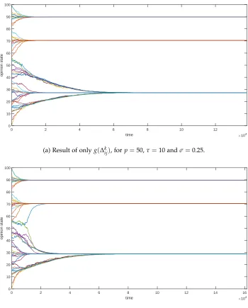
(a) Result of onlyg(∆k_ij), forp=50,τ=10 andσ=1.

0 0.5 1 1.5 2 2.5 3 3.5 4 4.5

time ×105

0 10 20 30 40 50 60 70 80 90 100

opinion state

(b) Result of onlyg(∆k_ij), forp=50,τ=10 andσ=0.5.

0 2 4 6 8 10 12

time ×104

0 10 20 30 40 50 60 70 80

opinion state

(a) Result of onlyg(∆k_ij), for p=50,τ=10 andσ=0.25.

0 2 4 6 8 10 12 14 16

time ×104

0 10 20 30 40 50 60 70 80 90 100

opinion state

(b) Result of onlyg(∆k_ij), forp=50,τ=10 andσ=0.1.

0 0.5 1 1.5 2 2.5 3

time _×105

0 10 20 30 40 50 60 70 80 90

opinion state

(a) Result of onlyh(ck_ij), for p=50 andτ=10.

0 10 20 30 40 50 60 70 80 90 100

initial opinions u 0

10 20 30 40 50 60 70 80 90 100

stabilized opinions

(b) Initial versus final opinions forp=50 andτ=10.

0 2 4 6 8 10 12 14

time ×105

0 10 20 30 40 50 60 70 80

opinion state

Table D.1: Statistical results for p=50.

τ accepted

hypothesis p-value

average number of stable clusters

std number of stable clusters

highest number of stable clusters

1 1 1,9780e-18 16 0 16

2 1 1,9780e-18 9,5400 4,3703 12

3 1 1,9780e-18 7,4600 1,8114 8

4 1 1,9780e-18 5,8600 1,8533 7

5 1 1,9780e-18 4,2100 1,4995 6

6 1 1,9780e-18 3,6600 1,9081 5

7 1 1,9780e-18 4,0700 1,4513 5

8 1 1,9780e-18 3,7200 1,1466 5

9 1 1,9780e-18 2,6900 1,1951 4

10 1 1,9780e-18 2,2900 0,9244 4

11 1 1,9780e-18 2,0500 0,6416 3

12 1 1,9780e-18 1,9100 0,5143 3

13 1 1,9780e-18 1,8500 0,6571 3

14 1 1,9780e-18 1,9000 0,4381 2

15 1 1,9780e-18 1,8500 0,5573 3

16 1 1,9780e-18 1,8900 0,4471 2

17 1 1,9780e-18 1,6500 0,6723 2

18 1 1,9780e-18 1,6600 0,6670 2

19 1 1,9780e-18 1,4500 0,7160 2

20 1 1,9780e-18 1,4000 0,6356 2

21 1 1,9780e-18 1,0900 0,3786 2

22 1 1,9780e-18 1,0100 0,1000 2

23 1 1,9780e-18 1 0 1

24 1 1,9780e-18 1 0 1

25 1 1,9780e-18 1 0 1

26 1 1,9780e-18 1 0 1

27 1 1,9780e-18 1 0 1

28 1 1,9780e-18 1 0 1

29 1 2,4434e-18 1 0 1

30 1 2,1396e-17 1 0 1

31 1 8,9881e-16 1 0 1

32 1 4,6649e-12 1 0 1

33 1 0,0117 1 0 1

34 0 0,9999 1 0 1

35 0 0,9999 1 0 1

36 0 1 1 0 1

37 0 1 1 0 1

38 0 1 1 0 1

39 0 1 1 0 1

40 0 1 1 0 1

41 0 1 1 0 1

42 0 1 1 0 1

43 0 1 1 0 1

44 0 1 1 0 1

45 0 1 1 0 1

46 0 1 1 0 1

47 0 1 1 0 1

48 0 1 1 0 1

Table E.1: Results for 100 simulations for each 1≤ τ ≤49, fork= 50. Table entries represent

intensities on the number of clusters that appeared, i.e., e.g. forτ=5 a result of 4 stable clusters

was observed 30 times.

number of clusters→

1 2 3 4 5 6 7 8 9 10 11 12 13 14 15 16

τ

↓

1 0 0 0 0 0 0 0 0 0 0 0 0 0 0 0 100

2 0 0 0 0 0 0 0 0 0 5 43 52 0 0 0 0

3 0 0 0 0 0 3 21 76 0 0 0 0 0 0 0 0

4 0 0 0 0 10 41 49 0 0 0 0 0 0 0 0 0

5 0 0 3 30 66 1 0 0 0 0 0 0 0 0 0 0

6 0 0 4 35 61 0 0 0 0 0 0 0 0 0 0 0

7 0 0 2 45 53 0 0 0 0 0 0 0 0 0 0 0

8 0 0 14 72 14 0 0 0 0 0 0 0 0 0 0 0

9 0 21 51 28 0 0 0 0 0 0 0 0 0 0 0 0

10 0 54 41 5 0 0 0 0 0 0 0 0 0 0 0 0

11 0 81 19 0 0 0 0 0 0 0 0 0 0 0 0 0

12 0 96 4 0 0 0 0 0 0 0 0 0 0 0 0 0

13 0 93 7 0 0 0 0 0 0 0 0 0 0 0 0 0

14 0 96 4 0 0 0 0 0 0 0 0 0 0 0 0 0

15 0 97 3 0 0 0 0 0 0 0 0 0 0 0 0 0

16 4 97 0 0 0 0 0 0 0 0 0 0 0 0 0 0

17 16 84 0 0 0 0 0 0 0 0 0 0 0 0 0 0

18 15 85 0 0 0 0 0 0 0 0 0 0 0 0 0 0

19 33 67 0 0 0 0 0 0 0 0 0 0 0 0 0 0

20 47 53 0 0 0 0 0 0 0 0 0 0 0 0 0 0

21 87 13 0 0 0 0 0 0 0 0 0 0 0 0 0 0

22 99 1 0 0 0 0 0 0 0 0 0 0 0 0 0 0

23 100 0 0 0 0 0 0 0 0 0 0 0 0 0 0 0

24 100 0 0 0 0 0 0 0 0 0 0 0 0 0 0 0

25 100 0 0 0 0 0 0 0 0 0 0 0 0 0 0 0

26 100 0 0 0 0 0 0 0 0 0 0 0 0 0 0 0

27 100 0 0 0 0 0 0 0 0 0 0 0 0 0 0 0

28 100 0 0 0 0 0 0 0 0 0 0 0 0 0 0 0

29 100 0 0 0 0 0 0 0 0 0 0 0 0 0 0 0

30 100 0 0 0 0 0 0 0 0 0 0 0 0 0 0 0

31 100 0 0 0 0 0 0 0 0 0 0 0 0 0 0 0

32 100 0 0 0 0 0 0 0 0 0 0 0 0 0 0 0

33 100 0 0 0 0 0 0 0 0 0 0 0 0 0 0 0

34 100 0 0 0 0 0 0 0 0 0 0 0 0 0 0 0

35 100 0 0 0 0 0 0 0 0 0 0 0 0 0 0 0

36 100 0 0 0 0 0 0 0 0 0 0 0 0 0 0 0

37 100 0 0 0 0 0 0 0 0 0 0 0 0 0 0 0

38 100 0 0 0 0 0 0 0 0 0 0 0 0 0 0 0

39 100 0 0 0 0 0 0 0 0 0 0 0 0 0 0 0

40 100 0 0 0 0 0 0 0 0 0 0 0 0 0 0 0

41 100 0 0 0 0 0 0 0 0 0 0 0 0 0 0 0

42 100 0 0 0 0 0 0 0 0 0 0 0 0 0 0 0

43 100 0 0 0 0 0 0 0 0 0 0 0 0 0 0 0

44 100 0 0 0 0 0 0 0 0 0 0 0 0 0 0 0

45 100 0 0 0 0 0 0 0 0 0 0 0 0 0 0 0

46 100 0 0 0 0 0 0 0 0 0 0 0 0 0 0 0

47 100 0 0 0 0 0 0 0 0 0 0 0 0 0 0 0

48 100 0 0 0 0 0 0 0 0 0 0 0 0 0 0 0

0

5

10

15

20

25

30

35

40

45

50

τ

0

10

20

30

40

50

60

70

80

90

100 _Intensity

1 cluster 2 clusters 3 clusters 4 clusters 5 clusters 6 clusters 7 clusters 8 clusters 10 clusters 11 clusters 12 clusters 16 clusters

0 2 4 6 8 10 12 14 16 18

time ×104

0 10 20 30 40 50 60 70 80 90 100

opinion state

(a) Typical opinion evolution for 50 agents, whereτ=15.

0 2 4 6 8 10

time ×105

0 10 20 30 40 50 60 70 80 90 100

opinion state

(b) Typical opinion evolution for 100 agents, whereτ=30.

0 2 4 6 8 10 12 14 16 18

time ×105

0 10 20 30 40 50 60 70 80 90 100

opinion state

(c) Typical opinion evolution for 200 agents, whereτ=60.