Improved testing for the efficiency of asset pricing theories in linear factor models

(1)

WORKING PAPERS SERIES

WP99-19

Improved Testing for the Efficiency

of Asset Pricing Theories in Linear

Factor Models

(2)

(3)

(4)

(5)

(6)

(7)

(8)

(9)

(10)

(11)

(12)

(13)

(14)

(15)

(16)

(17)

(18)

(19)

(20)

(21)

Table 1 Comparison of New Test Statistics and F-Statistics

A. Number of Observations T=60, Number of Factors K=1

Number of Test Statistics Percentile of Test Statistics

Assets (N) 0.5% 1.0% 2.5% 5.0% 10.0%

N=10 New Test Statistics 2.719 2.508 2.186 1.931 1.674

F(10,49) N=10, T-N-K=49 2.985 2.728 2.341 2.033 1.737

F(20,39) N=20, T-N-K=39 2.573 2.393 2.092 1.860 1.614

F(30,29) N=30, T-N-K=29 2.614 2.424 2.109 1.869 1.620

F(40,19) N=40, T-N-K=19 3.044 2.764 2.346 2.033 1.729

F(50,9) N=50, T-N-K=9 5.261 4.424 3.453 2.766 2.201

N=+infinite New Test Statistics 1.036 1.036 1.036 1.036 1.036 Notes: For the new test statistics, see equation (12). The new statistics are the average value of N different

F(1, T-K-1) distributions. The statistics reported in the table are the results of simulations with 10,000 replications. Detail simulation procedures are explained in section 3.1.

(22)

B. Number of Observations T=60, Number of Factors K=3

Assets (N) 0.5% 1.0% 2.5% 5.0% 10.0%

F(10,45) N=10, T-N-K=45 3.007 2.746 2.350 2.040 1.743

F(20,35) N=20, T-N-K=35 2.608 2.423 2.113 1.870 1.624

F(30,25) N=30, T-N-K=25 2.681 2.484 2.152 1.900 1.642

F(40,15) N=40, T-N-K=15 3.275 2.946 2.465 2.119 1.782

F(50,5) N=50, T-N-K=5 7.042 5.776 4.280 3.284 2.508

(23)

C. Number of Observations T=60, Number of Factors K=5

Assets (N) 0.5% 1.0% 2.5% 5.0% 10.0%

F(10,45) N=10, T-N-K=45 3.032 2.773 2.368 2.053 1.750

F(20,35) N=20, T-N-K=35 2.649 2.461 2.139 1.890 1.636

F(30,25) N=30, T-N-K=25 2.747 2.547 2.201 1.932 1.664

F(40,15) N=40, T-N-K=15 3.543 3.161 2.610 2.222 1.847

F(50,5) N=50, T-N-K=5 11.896 9.265 6.272 4.420 3.135

(24)

D. Number of Observations T=120, Number of Factors K=1

Assets (N) 0.5% 1.0% 2.5% 5.0% 10.0%

F(10,109) N=10, T-N-K=109 2.682 2.499 2.184 1.934 1.663

F(20,99) N=20, T-N-K=99 2.201 2.070 1.858 1.682 1.496

F(30,89) N=30, T-N-K=89 2.015 1.906 1.722 1.575 1.421

F(40,79) N=40, T-N-K=79 1.959 1.853 1.671 1.538 1.397

F(50,69) N=50, T-N-K=69 1.950 1.839 1.656 1.527 1.388

F(60,59) N=60, T-N-K=59 1.963 1.843 1.673 1.540 1.397

F(70,49) N=70, T-N-K=49 2.024 1.893 1.709 1.571 1.424

F(80,39) N=80, T-N-K=39 2.141 1.985 1.777 1.621 1.459

F(90,29) N=90, T-N-K=29 2.389 2.176 1.914 1.730 1.526

F(100,19) N=100, T-N-K=19 2.998 2.644 2.226 1.957 1.685

F(110,9) N=110, T-N-K=9 5.666 4.531 3.418 2.797 2.207

(25)

E. Number of Observations T=120, Number of Factors K=3

Assets (N) 0.5% 1.0% 2.5% 5.0% 10.0%

F(10,107) N=10, T-N-K=107 2.686 2.502 2.187 1.933 1.663

F(20,97) N=20, T-N-K=97 2.209 2.078 1.861 1.684 1.496

F(30,87) N=30, T-N-K=87 2.021 1.911 1.728 1.579 1.425

F(40,77) N=40, T-N-K=77 1.964 1.857 1.676 1.544 1.401

F(50,67) N=50, T-N-K=67 1.965 1.849 1.667 1.532 1.393

F(60,57) N=60, T-N-K=57 1.982 1.857 1.683 1.547 1.404

F(70,47) N=70, T-N-K=47 2.048 1.913 1.722 1.584 1.434

F(80,37) N=80, T-N-K=37 2.192 2.021 1.803 1.641 1.473

F(90,27) N=90, T-N-K=27 2.468 2.231 1.957 1.762 1.550

F(100,17) N=100, T-N-K=17 3.244 2.815 2.335 2.038 1.739

F(110,7) N=110, T-N-K=7 8.013 5.976 4.224 3.322 2.510

(26)

F. Number of Observations T=120, Number of Factors K=5

Assets (N) 0.5% 1.0% 2.5% 5.0% 10.0%

F(10,105) N=10, T-N-K=105 2.690 2.506 2.189 1.934 1.665

F(20,95) N=20, T-N-K=95 2.214 2.085 1.866 1.690 1.499

F(30,85) N=30, T-N-K=85 2.017 1.912 1.730 1.580 1.429

F(40,75) N=40, T-N-K=75 1.970 1.853 1.675 1.545 1.401

F(50,65) N=50, T-N-K=65 1.973 1.854 1.672 1.539 1.399

F(60,55) N=60, T-N-K=55 2.002 1.871 1.693 1.554 1.408

F(70,45) N=70, T-N-K=45 2.080 1.934 1.738 1.596 1.441

F(80,35) N=80, T-N-K=35 2.222 2.052 1.829 1.663 1.488

F(90,25) N=90, T-N-K=25 2.557 2.308 2.003 1.797 1.574

F(100,15) N=100, T-N-K=15 3.453 3.022 2.471 2.135 1.802

F(110,5) N=110, T-N-K=5 14.562 9.701 6.138 4.491 3.158

(27)

G. Number of Observations T=600, Number of Factors K=3

Assets (N) 0.5% 1.0% 2.5% 5.0% 10.0%

F(10,587) N=10, T-N-K=587 2.556 2.366 2.061 1.837 1.600

F(20,577) N=20, T-N-K=577 2.071 1.930 1.738 1.599 1.442

F(30,567) N=30, T-N-K=567 1.825 1.718 1.579 1.468 1.348

F(40,557) N=40, T-N-K=557 1.719 1.622 1.518 1.422 1.318

F(50,547) N=50, T-N-K=547 1.629 1.564 1.469 1.387 1.286

F(60,537) N=60, T-N-K=537 1.603 1.515 1.418 1.341 1.262

F(70,527) N=70, T-N-K=527 1.546 1.483 1.387 1.318 1.236

F(80,517) N=80, T-N-K=517 1.494 1.445 1.369 1.303 1.226

F(90,507) N=90, T-N-K=507 1.493 1.427 1.344 1.288 1.219

F(100,497) N=100, T-N-K=497 1.470 1.418 1.339 1.282 1.211

F(110,487) N=110, T-N-K=487 1.448 1.405 1.329 1.263 1.197

F(200,397) N=200, T-N-K=397 1.371 1.322 1.268 1.216 1.167

F(500,97) N=500, T-N-K=97 1.541 1.483 1.388 1.316 1.238

(28)

[image:28.595.82.516.240.596.2]

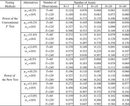
Table 2 Power of the Conventional F

Test and the New Test of the CAPM

for the Hypothesis H

0

: a=0, H

1

: a=

m

.

Testing Alternatives Number of Number of Assets

Methods Observations N=1 N=5 N=10 N=20 N=40

µp=8.5% T=60 0.124 0.076 0.066 0.061 0.052

!p=16% T=120 0.189 0.101 0.083 0.073 0.060

Power of the T=240 0.344 0.172 0.135 0.100 0.082

Conventional µp=10.2% T=60 0.196 0.105 0.084 0.069 0.056

F Test !p=16% T=120 0.327 0.172 0.124 0.098 0.073

T=240 0.598 0.333 0.251 0.169 0.120 µp=11.6% T=60 0.272 0.135 0.101 0.079 0.060

!p=16% T=120 0.456 0.252 0.171 0.129 0.091

T=240 0.771 0.497 0.378 0.258 0.170 µp=13.0% T=60 0.339 0.169 0.121 0.091 0.064

!p=16% T=120 0.575 0.333 0.225 0.161 0.107

T=240 0.877 0.636 0.507 0.349 0.227 µp=8.5% T=60 0.124 0.077 0.068 0.061 0.057

!p=16% T=120 0.189 0.103 0.088 0.078 0.069

T=240 0.344 0.180 0.132 0.111 0.088 µp=10.2% T=60 0.196 0.110 0.087 0.074 0.066

Power of !p=16% T=120 0.327 0.172 0.138 0.110 0.088

the New Test T=240 0.598 0.340 0.242 0.188 0.137

µp=11.6% T=60 0.272 0.145 0.108 0.089 0.077

!p=16% T=120 0.456 0.246 0.196 0.145 0.112

T=240 0.771 0.507 0.372 0.278 0.192 µp=13.0% T=60 0.339 0.183 0.132 0.102 0.086

!p=16% T=120 0.575 0.325 0.260 0.188 0.138

T=240 0.877 0.647 0.502 0.384 0.264 Notes: The table reports simulation results on the case of the null hypothesis H0:aj=0, j=1,…,N

against H1:aj=µ, j=1,…,N. The non-central variables of the F test and the new test are represented

(29)

[image:29.612.50.562.258.374.2]

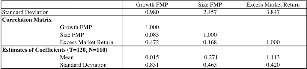
Table 3 Properties of Factors and Their Regression Coefficients

A. Entire Sample Period (April 1989 - March 1999)

Growth FMP Size FMP Excess Market Return

Standard Deviation 0.980 2.457 3.847

Correlation Matrix

Growth FMP 1.000

Size FMP 0.083 1.000

Excess Market Return 0.472 0.168 1.000

Estimates of Coefficients (T=120, N=110)

Mean 0.015 -0.271 1.113

B. Second Half Sample Period (April 1994 - March 1999)

Growth FMP Size FMP Excess Market Return

Correlation Matrix

Growth FMP 1.000

Size FMP 0.075 1.000

Excess Market Return 0.550 0.102 1.000

Estimates of Coefficients (T=60, N=50)

Mean -0.109 -0.246 0.980

Notes: All factor returns are monthly log-returns and have the expected value of zero.

The entire sample preiod (Panel A) is used for T=120, and the second half sample period (Panel B)

(30)

[image:30.842.58.782.99.498.2]

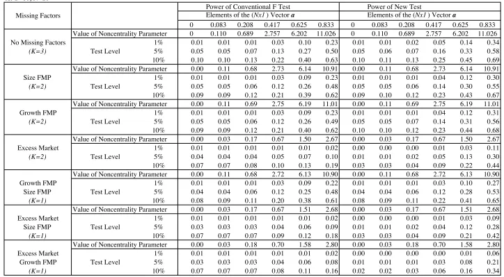
Table 4 Power of the Conventional F

Test and the New Test of Linear Factor Model for the Null Hypothesis H

0 M

: a=0

against the Alternative Hypothesis H

1

M

: a=

m

in the Presence of Missing Factors

A. T=60, N=10

Power of Conventional F Test Power of New Test

Missing Factors Elements of the (Nx1) Vector a Elements of the (Nx1) Vector a

0 0.083 0.208 0.417 0.625 0.833 0 0.083 0.208 0.417 0.625 0.833 Value of Noncentrality Parameter 0 0.110 0.689 2.757 6.202 11.026 0 0.110 0.689 2.757 6.202 11.026

No Missing Factors 1% 0.01 0.01 0.01 0.03 0.10 0.23 0.01 0.01 0.02 0.05 0.14 0.34

(K=3) Test Level 5% 0.05 0.05 0.07 0.13 0.27 0.50 0.05 0.06 0.07 0.16 0.33 0.58

10% 0.10 0.10 0.13 0.22 0.40 0.63 0.10 0.11 0.13 0.25 0.45 0.69 Value of Noncentrality Parameter 0.00 0.11 0.68 2.73 6.14 10.91 0.00 0.11 0.68 2.73 6.14 10.91

Size FMP 1% 0.01 0.01 0.01 0.03 0.09 0.23 0.01 0.01 0.01 0.04 0.12 0.30

(K=2) Test Level 5% 0.05 0.05 0.06 0.12 0.26 0.48 0.05 0.05 0.06 0.14 0.30 0.55

Growth FMP 1% 0.01 0.01 0.01 0.03 0.09 0.23 0.01 0.01 0.01 0.04 0.12 0.31

(K=2) Test Level 5% 0.05 0.05 0.06 0.12 0.26 0.49 0.05 0.05 0.07 0.14 0.31 0.56

Excess Market 1% 0.01 0.01 0.01 0.01 0.01 0.02 0.00 0.00 0.00 0.01 0.03 0.11

(K=2) Test Level 5% 0.04 0.04 0.04 0.05 0.07 0.10 0.01 0.01 0.02 0.05 0.13 0.30

Growth FMP 1% 0.01 0.01 0.01 0.03 0.09 0.22 0.01 0.01 0.01 0.03 0.10 0.27

Size FMP Test Level 5% 0.04 0.04 0.06 0.12 0.25 0.48 0.04 0.04 0.06 0.12 0.28 0.53

(K=1) 10% 0.08 0.09 0.11 0.20 0.38 0.61 0.08 0.09 0.11 0.22 0.41 0.65

Value of Noncentrality Parameter 0.00 0.03 0.17 0.67 1.51 2.68 0.00 0.03 0.17 0.67 1.51 2.68

Excess Market 1% 0.01 0.01 0.01 0.01 0.01 0.02 0.00 0.00 0.00 0.01 0.03 0.09

(K=1) 10% 0.07 0.07 0.07 0.09 0.12 0.18 0.03 0.03 0.04 0.09 0.21 0.42

Excess Market 1% 0.01 0.01 0.01 0.01 0.01 0.02 0.00 0.00 0.00 0.00 0.01 0.06

Growth FMP Test Level 5% 0.03 0.03 0.03 0.04 0.06 0.08 0.01 0.01 0.01 0.03 0.08 0.21

(K=1) 10% 0.07 0.07 0.07 0.08 0.11 0.16 0.02 0.02 0.03 0.06 0.16 0.34

Notes: Randomly selected N excess equity returns included in S&P500 are estimated with three factors in the linear regression model; excess market return, size and growth FMP returns. Then the coefficients and the variance of disturbance terms are used to generate N excess equity returns, which are used to test the power of the F test and our new test in the presence of missing factors. See section 3.2 for a detailed explanation on the simulation proceddure. The numbers in 'Elements of

the (Nx1) Vector a' are monthly returns equivalent to 0%, 1%, 2.5%, 5%, 7.5%, and 10% in annual term. T=60 represents 60 monthly returns from April 1994 to March 1999.

(31)

B. T=60, N=50

(K=3) Test Level 5% 0.05 0.06 0.06 0.10 0.17 0.29 0.05 0.06 0.11 0.37 0.82 0.99

Size FMP 1% 0.01 0.01 0.01 0.02 0.04 0.09 0.01 0.01 0.02 0.13 0.56 0.94

(K=2) Test Level 5% 0.05 0.05 0.06 0.10 0.18 0.31 0.04 0.04 0.08 0.31 0.78 0.98

Growth FMP 1% 0.01 0.01 0.01 0.02 0.05 0.10 0.01 0.01 0.02 0.14 0.57 0.95

(K=2) Test Level 5% 0.05 0.05 0.06 0.10 0.19 0.32 0.04 0.05 0.09 0.32 0.79 0.99

Excess Market 1% 0.01 0.01 0.01 0.01 0.02 0.02 0.00 0.00 0.00 0.01 0.16 0.68

(K=2) Test Level 5% 0.05 0.05 0.05 0.05 0.07 0.09 0.00 0.00 0.01 0.06 0.38 0.87

Growth FMP 1% 0.01 0.01 0.01 0.02 0.05 0.11 0.00 0.01 0.01 0.10 0.50 0.93

(K=1) 10% 0.09 0.10 0.12 0.18 0.31 0.51 0.06 0.07 0.12 0.40 0.84 0.99

Excess Market 1% 0.01 0.01 0.01 0.01 0.02 0.02 0.00 0.00 0.00 0.01 0.13 0.63

(K=1) 10% 0.09 0.09 0.10 0.11 0.13 0.17 0.00 0.01 0.01 0.09 0.48 0.91

Excess Market 1% 0.01 0.01 0.01 0.01 0.01 0.02 0.00 0.00 0.00 0.00 0.06 0.46

(K=1) 10% 0.09 0.09 0.09 0.10 0.12 0.15 0.00 0.00 0.00 0.05 0.33 0.83

Notes: Randomly selected N excess equity returns included in S&P500 are estimated with three factors in the linear regression model; excess market return, size and growth FMP returns. Then the coefficients and the variance of disturbance terms are used to generate

N excess equity returns, which are used to test the power of the F test and our new test in the presence of missing factors.

See section 3.2 for a detailed explanation on the simulation proceddure. The numbers in 'Elements of the (Nx1) Vector a' are monthly returns equivalent to 0%, 1%, 2.5%, 5%, 7.5%, and 10% in annual term. T=60 represents 60 monthly returns from April 1994 to March 1999.

(32)

C. T=120, N=10

(K=3) Test Level 5% 0.05 0.05 0.08 0.24 0.56 0.86 0.05 0.06 0.10 0.28 0.61 0.90

Size FMP 1% 0.01 0.01 0.02 0.09 0.31 0.66 0.01 0.01 0.02 0.10 0.35 0.72

(K=2) Test Level 5% 0.04 0.05 0.08 0.23 0.55 0.85 0.04 0.05 0.08 0.25 0.58 0.88

Growth FMP 1% 0.01 0.01 0.02 0.09 0.31 0.66 0.01 0.01 0.02 0.10 0.35 0.72

(K=2) Test Level 5% 0.04 0.05 0.08 0.24 0.55 0.85 0.04 0.05 0.08 0.25 0.58 0.88

Excess Market 1% 0.01 0.01 0.01 0.01 0.02 0.05 0.00 0.00 0.00 0.02 0.12 0.40

(K=2) Test Level 5% 0.03 0.03 0.04 0.05 0.10 0.20 0.01 0.01 0.02 0.08 0.30 0.66

Growth FMP 1% 0.01 0.01 0.02 0.08 0.30 0.66 0.01 0.01 0.02 0.09 0.32 0.69

(K=1) 10% 0.09 0.10 0.14 0.36 0.68 0.92 0.09 0.10 0.14 0.36 0.70 0.93

Excess Market 1% 0.01 0.01 0.01 0.01 0.02 0.05 0.00 0.00 0.00 0.02 0.10 0.37

(K=1) 10% 0.07 0.07 0.07 0.11 0.18 0.32 0.02 0.03 0.04 0.15 0.43 0.78

Excess Market 1% 0.01 0.01 0.01 0.01 0.02 0.04 0.00 0.00 0.00 0.01 0.07 0.31

(K=1) 10% 0.07 0.07 0.07 0.10 0.17 0.29 0.02 0.02 0.03 0.12 0.37 0.73

(33)

D. T=120, N=110

(K=3) Test Level 5% 0.05 0.05 0.07 0.14 0.29 0.52 0.05 0.07 0.25 0.94 1.00 1.00

Size FMP 1% 0.01 0.01 0.01 0.03 0.09 0.21 0.01 0.01 0.06 0.78 1.00 1.00

(K=2) Test Level 5% 0.05 0.05 0.06 0.14 0.31 0.55 0.03 0.05 0.20 0.92 1.00 1.00

Growth FMP 1% 0.01 0.01 0.01 0.03 0.10 0.23 0.01 0.01 0.08 0.80 1.00 1.00

(K=2) Test Level 5% 0.05 0.05 0.07 0.15 0.33 0.58 0.04 0.06 0.23 0.93 1.00 1.00

Excess Market 1% 0.01 0.01 0.01 0.01 0.02 0.02 0.00 0.00 0.00 0.13 0.96 1.00

(K=2) Test Level 5% 0.05 0.05 0.05 0.06 0.07 0.10 0.00 0.00 0.00 0.33 0.99 1.00

Growth FMP 1% 0.01 0.01 0.01 0.03 0.10 0.25 0.01 0.01 0.06 0.77 1.00 1.00

(K=1) 10% 0.09 0.10 0.13 0.27 0.52 0.78 0.07 0.09 0.30 0.96 1.00 1.00

Excess Market 1% 0.01 0.01 0.01 0.01 0.01 0.02 0.00 0.00 0.00 0.11 0.95 1.00

(K=1) 10% 0.09 0.09 0.10 0.11 0.14 0.18 0.00 0.00 0.01 0.44 1.00 1.00

Excess Market 1% 0.01 0.01 0.01 0.01 0.02 0.02 0.00 0.00 0.00 0.06 0.89 1.00

(K=1) 10% 0.09 0.09 0.09 0.11 0.14 0.18 0.00 0.00 0.00 0.30 0.99 1.00

(34)

E. T=60, N=110

Power of New Test

Missing Factors Elements of the (Nx1) Vector a

0 0.083 0.208 0.417 0.625 0.833

Value of Noncentrality Parameter 0 1.195 7.469 29.876 67.221 119.503

No Missing Factors 1% 0.01 0.01 0.04 0.32 0.90 1.00

(K=3) Test Level 5% 0.05 0.06 0.13 0.56 0.97 1.00

10% 0.10 0.12 0.22 0.69 0.99 1.00

Value of Noncentrality Parameter 0.00 1.10 6.88 27.53 61.93 110.10

Size FMP 1% 0.01 0.01 0.03 0.27 0.88 1.00

(K=2) Test Level 5% 0.04 0.05 0.10 0.50 0.96 1.00

10% 0.08 0.09 0.17 0.64 0.98 1.00

Growth FMP 1% 0.01 0.01 0.03 0.29 0.89 1.00

(K=2) Test Level 5% 0.04 0.05 0.11 0.53 0.97 1.00

10% 0.09 0.10 0.19 0.66 0.99 1.00

Excess Market 1% 0.00 0.00 0.00 0.01 0.32 0.94

(K=2) Test Level 5% 0.00 0.00 0.00 0.05 0.56 0.99

10% 0.00 0.00 0.00 0.11 0.70 1.00

Growth FMP 1% 0.00 0.00 0.02 0.20 0.83 1.00

Size FMP Test Level 5% 0.03 0.03 0.08 0.45 0.95 1.00

(K=1) 10% 0.06 0.07 0.14 0.58 0.98 1.00

Excess Market 1% 0.00 0.00 0.00 0.01 0.23 0.91

Size FMP Test Level 5% 0.00 0.00 0.00 0.04 0.50 0.98

(K=1) 10% 0.00 0.00 0.00 0.08 0.64 0.99

Excess Market 1% 0.00 0.00 0.00 0.00 0.09 0.75

Growth FMP Test Level 5% 0.00 0.00 0.00 0.01 0.27 0.92

(K=1) 10% 0.00 0.00 0.00 0.02 0.41 0.96

N excess equity returns, which are used to test the power of the new test in the presence of missing factors.

See section 3.2 for a detailed explanation on the simulation proceddure. The numbers in 'Elements of the (Nx1) Vector a' are monthly returns equivalent to 0%, 1%, 2.5%, 5%, 7.5%, and 10% in annual term. T=60 represents 60 monthly returns from April 1994 to March 1999. Note that the conventional F test is not available in this case. K is the number of factors used for the power test.

(35)

[image:35.595.64.528.107.735.2]

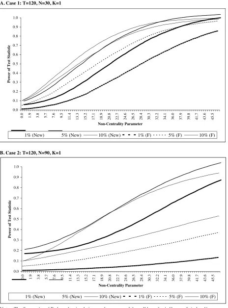
Figure 1 Power of the New and F

(N, T-N-K

) Test Statistics for the Null Hypothesis

H

0

: a

j

=0

for all j

against the Alternative Hypothesis H

1

: a

1

=

m

and a

j

=0 for j

>1:

A. Case 1: T=120, N=30, K=1

B. Case 2: T=120, N=90, K=1

Notes: The figures A and B show the simulation results on case of the null hypothesis H0:aj=0, j=1,...,N

against the alternative hypothesis H1:aj=µ, for j=1, and aj=0, for j=2,...,N. Simulation procedures

are explained in section 3.2. The non-central variables for the alternative hypothesis are generated with equations (24) and (25) for the conventional F test and the new test, respectively.

0.0 0.1 0.2 0.3 0.4 0.5 0.6 0.7 0.8 0.9 1.0

0.0 1.9 3.8 5.7 7.6 9.5 _11.4 _13.3 _15.2 _17.1 _18.9 _20.8 _22.7 _24.6 _26.5 _28.4 _30.3 _32.2 _34.1 _36.0 _37.9 _39.8 _41.7 _43.6 _45.5

Non-Centrality Parameter P o w er o f T es t S ta ti st ic

1% (New) 5% (New) 10% (New) 1% (F) 5% (F) 10% (F) 0.0 0.1 0.2 0.3 0.4 0.5 0.6 0.7 0.8 0.9 1.0

0.0 1.9 3.8 5.7 7.6 9.5 _11.4 _13.3 _15.2 _17.1 _18.9 _20.8 _22.7 _24.6 _26.5 _28.4 _30.3 _32.2 _34.1 _36.0 _37.9 _39.8 _41.7 _43.6 _45.5

Non-Centrality Parameter P o w er o f T es t S ta ti st ic

(36)

!

**_{!"#$%&'()*)+#,(,+#%+,(}**

(

List of other working papers:

1999

1. Yin-Wong Cheung, Menzie Chinn and Ian Marsh, How do UK-Based Foreign Exchange Dealers Think Their Market Operates?, WP99-21

2. Soosung Hwang, John Knight and Stephen Satchell, Forecasting Volatility using LINEX Loss Functions, WP99-20

3. Soosung Hwang and Steve Satchell, Improved Testing for the Efficiency of Asset Pricing Theories in Linear Factor Models, WP99-19

4. Soosung Hwang and Stephen Satchell, The Disappearance of Style in the US Equity Market, WP99-18

5. Soosung Hwang and Stephen Satchell, Modelling Emerging Market Risk Premia Using Higher Moments, WP99-17

6. Soosung Hwang and Stephen Satchell, Market Risk and the Concept of Fundamental Volatility: Measuring Volatility Across Asset and Derivative Markets and Testing for the Impact of Derivatives Markets on Financial Markets, WP99-16

7. Soosung Hwang, The Effects of Systematic Sampling and Temporal Aggregation on Discrete Time Long Memory Processes and their Finite Sample Properties, WP99-15

8. Ronald MacDonald and Ian Marsh, Currency Spillovers and Tri-Polarity: a Simultaneous Model of the US Dollar, German Mark and Japanese Yen, WP99-14

9. Robert Hillman, Forecasting Inflation with a Non-linear Output Gap Model, WP99-13

10.Robert Hillman and Mark Salmon , From Market Micro-structure to Macro Fundamentals: is there Predictability in the Dollar-Deutsche Mark Exchange Rate?, WP99-12

11.Renzo Avesani, Giampiero Gallo and Mark Salmon, On the Evolution of Credibility and Flexible Exchange Rate Target Zones, WP99-11

12.Paul Marriott and Mark Salmon, An Introduction to Differential Geometry in Econometrics, WP99-10

13.Mark Dixon, Anthony Ledford and Paul Marriott, Finite Sample Inference for Extreme Value Distributions, WP99-09

14.Ian Marsh and David Power, A Panel-Based Investigation into the Relationship Between Stock Prices and Dividends, WP99-08

15.Ian Marsh, An Analysis of the Performance of European Foreign Exchange Forecasters, WP99-07

16.Frank Critchley, Paul Marriott and Mark Salmon, An Elementary Account of Amari's Expected Geometry, WP99-06

17.Demos Tambakis and Anne-Sophie Van Royen, Bootstrap Predictability of Daily Exchange Rates in ARMA Models, WP99-05

18.Christopher Neely and Paul Weller, Technical Analysis and Central Bank Intervention, WP99-04

19.Christopher Neely and Paul Weller, Predictability in International Asset Returns: A Re-examination, WP99-03

20.Christopher Neely and Paul Weller, Intraday Technical Trading in the Foreign Exchange Market, WP99-02

21.Anthony Hall, Soosung Hwang and Stephen Satchell, Using Bayesian Variable Selection Methods to Choose Style Factors in Global Stock Return Models, WP99-01

1998

1. Soosung Hwang and Stephen Satchell, Implied Volatility Forecasting: A Compaison of Different Procedures Including Fractionally Integrated Models with Applications to UK Equity Options, WP98-05

(37)

4. Adam Kurpiel and Thierry Roncalli , Option Hedging with Stochastic Volatility, WP98-02