Hydraulic models in stream restoration

Full text

(1)20-10-2016. Master thesis. Hydraulic models in stream restoration. 1. Ruud Boom.

(2) 2.

(3) MSc thesis Faculty of Engineering Technology Water Engineering & Management University of Twente. Hydraulic models in stream restoration. Author R.J.H.M. Boom BSc.. External supervisors Dr. Ir. A.J. Paarlberg HKV Lijn in Water. Graduation supervisor Dr. Ir. D.C.M. Augustijn University of Twente. Ir. H.J. Barneveld HKV Lijn in Water. Daily supervisor Ir. R.P. van Denderen University of Twente. Ir. C. Huising Waterschap Vallei & Veluwe Ing. E. Raaijmakers Waterschap Peel & Maasvallei. 3.

(4) 4.

(5) Abstract Water boards perform stream restoration projects mainly to restore ecology. Hydrodynamic modelling is an important part of those restoration projects, mainly to forecast future water levels and flood risk. In Dutch stream restoration projects, it is very common to use one-dimensional Sobek software for hydrodynamic modelling. Still, though monitoring of stream restoration projects is scarcely performed, it is a common belief that hydraulic forecasts are not always optimal. The general assumption is that multi-dimensional models can improve upon the predictions made with the one-dimensional model. This research makes a comparison between modelling stream restoration projects in their design phase with onedimensional Sobek software compared to two-dimensional Delft3D FM software. The Delft3D FM software was specifically selected out of the two-dimensional models available, because of its flexible grid. This means both spacing and shape of the grid can vary, which is especially useful in modelling meandering streams. The objective of the research was: to determine if modelling stream restoration projects, in their design phase, with a two-dimensional (Delft3D FM) compared to a one-dimensional (Sobek) model has advantages in forecasting water levels and developments in morphology and vegetation. To investigate this, two restoration projects were modelled, one in the Lunterse beek and one in the Tungelroyse beek. Both projects were traditional stream restoration projects (re-meandering projects). For the stream restoration project analysed in the Lunterse beek two models were set-up, a Sobek model and a Delft3D FM model. Both models were set-up for the period shortly after restoration and stationary discharge scenarios were used as model forcing. A comparison between simulated water levels and observed water levels showed that the one-dimensional model performed better than the two-dimensional model for this particular situation. It was also found that the water level simulations with the Delft3D FM model could improve if lower roughness values were selected or if the bed level interpolation method was changed though, which was not the case for the Sobek model. It was found that differences in output between the models were likely caused by differences in bathymetry and experience in working with the models. For the stream restoration project performed in the Tungelroyse beek, a Delft3D FM model was set-up. Again, the period shortly after restoration was modelled using stationary discharge scenarios as forcing for the model. Performance of water level forecasts improved compared to the Delft3D FM model of the Lunterse beek. However, it was concluded that advantages of a two-dimensional model over a one-dimensional model will likely not come from water level forecasts since the water levels simulated with the Sobek model are already accurate. It is expected that the two-dimensional model can list equally good results though if more experience is gained with twodimensional modelling in stream restoration projects. Forecasts in morphological developments were made based upon output of the Delft3D FM models. First the locations where transport can be expected were determined using the Shields parameter and the critical Shields parameter. After that flow velocity and flow direction maps were made for the most important discharge scenarios. For the Lunterse beek these maps were qualitatively compared to monitored quantitative developments in bed level. The maps created with the high uniform discharge scenarios (T100, T10 and T1) showed good correspondence to monitored developments, while the lower discharge scenarios (T0.05 and T0.005) showed some correspondence looking into bed erosion and sedimentation. It was found that the monitored discharge for the given period was between the discharge used as forcing for the T0.05 and T0.005 scenarios. The bank erosion that was monitored in the field could not be explained by these scenarios. An explanation for this can be that water levels are overestimated in the model, wherefore flow velocities are underestimated for equal discharges. The flow velocity and flow direction maps made for the Tungelroyse beek agreed with qualitative developments monitored with respect to morphology. However, no quantitative measurements were performed of bed level developments. Therefore, agreement between forecasts made with the models and developments encountered in reality could not be proven. In the end it was concluded that there might be benefits of a two-dimensional model with respect to forecasting morphological developments after stream restoration in its design phase, but this could not be proven in this research. To make forecasts about expected developments in vegetation, flow velocity output of the Delft3D FM models was used. In the literature it was found that more vegetation can be expected for locations with low flow velocities and less vegetation if flow velocities are high. Though developments in vegetation depend on many other factors, it was found that forecasts corresponded quite well to monitored developments in vegetation for some scenarios. Validation was performed for the Lunterse beek by using a high resolution aerial image and for the Tungelroyse beek using a Normalized Difference Vegetation Index (NDVI) map. It has to be noted though that in-stream vegetation developments could not be validated, while these are often very important for water boards. Finally it was concluded that using a two-dimensional Delft3D FM model in the design phase of stream restoration projects to make forecasts in vegetation development might be beneficial. Using flow velocity output of the twodimensional model to base these forecasts upon gave good results for a few discharge scenarios for both streams. There might also be a benefit in two-dimensional modelling with respect to making forecasts in morphological 5.

(6) developments, however this is only partly supported by this research. Finally, it became clear that advantages of a two-dimensional model compared to one-dimensional model are likely not present in water level forecasts since the one-dimensional model already performs very well. It is expected though, that the water level forecasts made with the two-dimensional model can be improved by gathering more experience. This should eventually lead to water level forecasts that are just as accurate for the two-dimensional model as for the one-dimensional model.. 6.

(7) Preface With this documentation I (hope to) finish my Master study Water Engineering and Management at the University of Twente. It is the same University where I started my Bachelor Civil Engineering a little over five years ago. This period has been of invaluable importance for me to develop myself into an engineer and to grow as a person. For this, I would like to thank everyone that contributed. This graduation project started at the 1 st of February 2016 and was performed mainly at HKV Lijn in Water in Lelystad. I would like to thank the company and all its employees for giving me the possibility to perform my thesis here and for creating a positive environment to do so. A special thanks goes out to my external supervisors Andries Paarlberg and Hermjan Barneveld from HKV for their help during the assignment. Besides that, I would like to thank my supervisors Erik Raaijmakers and Christian Huising from Water board Peel & Maasvallei and Water board Vallei & Veluwe respectively. They helped to collect all the data needed for this research and provided tons of site-specific information. A thanks also goes out to Arthur van Dam from Deltares for helping out with questions about the Delft3D FM software. For the high resolution aerial photo of the Lunterse beek I would like to thank the Unmanned Aerial Remote Sensing Facility of the Wageningen University (WUR-UARSF) and the Section of Environmental Fluid Mechanics from the Delft University of Technology, and in particular Andrés Vargas Luna for letting me use this photo. Finally, I would like to thank Denie Augustijn and Pepijn van Denderen from the University of Twente for their supervision and feedback during the Master thesis.. 7.

(8) Table of contents Abstract ................................................................................................................................................................... 5 Preface .................................................................................................................................................................... 7 1.. 2.. 3.. Introduction ................................................................................................................................................... 10 1.1. General background............................................................................................................................. 10. 1.2. Problem definition ................................................................................................................................ 10. 1.3. Objective and research questions ........................................................................................................ 11. 1.4. Reading guide ...................................................................................................................................... 11. Stream restoration and case studies............................................................................................................. 12 2.1. Stream restoration................................................................................................................................ 12. 2.2. The Lunterse beek ............................................................................................................................... 12. 2.3. The Tungelroyse beek ......................................................................................................................... 14. Methodology: model set-up........................................................................................................................... 17 3.1. General ................................................................................................................................................ 17. 3.2. Discharge scenarios, Q-h relations and validation locations ................................................................ 17. 3.2.1. Lunterse beek .................................................................................................................................. 17. 3.2.2. Tungelroyse beek ............................................................................................................................ 20. 3.3. 4.. Structures ............................................................................................................................................. 24. 3.3.1. Lunterse beek .................................................................................................................................. 24. 3.3.2. Tungelroyse beek ............................................................................................................................ 25. 3.4. Sobek model Lunterse beek ................................................................................................................ 26. 3.5. Delft3D FM model Lunterse beek......................................................................................................... 29. 3.6. Delft3D FM model Tungelroyse beek ................................................................................................... 31. Methodology: morphology and vegetation .................................................................................................... 35 4.1. Morphological developments ............................................................................................................... 35. 4.1.1 General ................................................................................................................................................ 35 4.1.2 Lunterse beek ...................................................................................................................................... 36 4.1.3 Tungelroyse beek ................................................................................................................................ 37 4.2 5.. 6.. Developments in vegetation ................................................................................................................. 38. Results Lunterse beek .................................................................................................................................. 40 5.1. Water levels ......................................................................................................................................... 40. 5.2. Morphological developments ............................................................................................................... 44. 5.3. Developments in vegetation ................................................................................................................. 48. Results Tungelroyse beek ............................................................................................................................ 50 6.1. Water levels ......................................................................................................................................... 50. 6.2. Morphological developments ............................................................................................................... 51. 6.3. Developments in vegetation ................................................................................................................. 55. 7.. Discussion .................................................................................................................................................... 57. 8.. Conclusions .................................................................................................................................................. 60. 9.. Recommendations ........................................................................................................................................ 62. Bibliography ........................................................................................................................................................... 64 Appendix A: Fitted Q-h relations Lunterse beek .................................................................................................... 67 Appendix B: Schematisation Tungelroyse beek with available data ...................................................................... 71 8.

(9) Appendix C: Fitted Q-h relations Tungelroyse beek .............................................................................................. 72 Appendix D: Sensitivity analysis Sobek Lunterse beek ......................................................................................... 74 Appendix E: Bed roughness Sobek ....................................................................................................................... 75 Appendix F: Test Surfis interpolations ................................................................................................................... 80 Appendix G: Difference AHN2 and measurements ............................................................................................... 83 Appendix H: Bed roughness Delft3D FM Lunterse beek ....................................................................................... 84 Appendix I: Sensitivity analysis Delft3D FM Lunterse beek ................................................................................... 86 Appendix J: Bed roughness Delft3D FM Tungelroyse beek .................................................................................. 92 Appendix K: Summary literature study vegetation ................................................................................................. 93 Appendix L: Straight channel tests ........................................................................................................................ 95. 9.

(10) 1. Introduction This chapter introduces the subject of this Master thesis. Section 1.1 gives a general background and explains why this research is of importance. In section 1.2 the problem is given, while the objective and research questions are presented in section 1.3. Finally, section 1.4 provides a reading guide.. 1.1. General background. Water systems in the Netherlands are under constant control and manipulation in order to serve water-related interests (Rijkswaterstaat, 2011). In the 20th century a lot of work was done to normalize streams and rivers in order to increase discharge capacities and decrease flooding (STOWA, 2015). The normalisation has shown to be effective in this, but downsides to these changes were underestimated. Normalization made discharging of streams too fast in many cases. Besides that, streams are deeper than before which caused decreases in groundwater levels. Finally, and most importantly, aquatic ecology is seriously affected by the normalization of streams and rivers, since variations in flow conditions are of vital importance for the survival of many organisms (Verdonschot et al., 2012). To counteract the negative effects of normalization, stream restoration projects are carried out. In these projects the focus is often on improving ecology and water quality (Didderen et al., 2009; Kail & Angelopoulos, 2014; Palmer & Allan, 2006). The stream restoration measure that is most often applied in the Netherlands is re-meandering, while in the rest of Europe the development of natural riparian vegetation is most popular (Didderen et al., 2009; Kail & Angelopoulos, 2014). When river or stream restoration projects are designed, setting up a hydrodynamic model is usually an integral and very valuable part of the project (Schwartz & Neff, 2011). Predicting future water levels and flood risks would be hardly possible without these models. Currently, one-dimensional hydrodynamic models are often preferred over multi-dimensional models due to the fact that multi-dimensional models are more resource intensive (Volkwein, 2011). Looking at water boards in particular, organisations that are often responsible for stream restoration, a lack of experience in working with multi-dimensional models further stimulates the choice for one-dimensional models in those projects. At the same time though, the general assumption is that multi-dimensional hydrodynamic models can give better hydraulic predictions than one-dimensional models (Jowett & Duncan, 2012). The use of multi-dimensional models is increasing though. The large rivers in the Netherlands are standardly modelled two- and sometimes even three-dimensionally nowadays (Sloff et al., 2012). In stream restoration projects however, one-dimensional flow models are still used most of the time. There is some research that has focussed on using two-dimensional models in these projects though. An example is the research of Zantvoort et al. (2008) that was targeted on investigating the added value of two-dimensional flow models in flood calculations. The research showed that two-dimensional modelling had many advantages over one-dimensional modelling when performing flood calculations. Regarding hydraulic modelling though, no studies were performed on comparing multi-dimensional with one-dimensional models. Stream restoration projects are an excellent opportunity for such an investigation. Since 2009, Deltares has been working on a new hydro software package. As a first step, they extended the Delft3D model with a flexible grid: Delft3D Flexible Mesh (Delft3D FM). The main advantage of this software is the possibility to generate a flexible grid in which both spacing and shape can vary (Deltares, 2013). This makes it possible to model the flow while using grids that do not conform to the matrix shape needed in curvilinear grids. Therefore the model software is more suited to capture important details. Especially in modelling meandering streams, where dimensions are often small and sinuosity can become large, the flexibility in the grid might be useful. This raises the question whether it is possible to better predict hydraulic effects of stream restoration measures using the relatively new two-dimensional Delft3D FM software compared to using a more traditional one-dimensional Sobek model as often done nowadays.. 1.2. Problem definition. Water boards are often responsible for stream restoration projects in the Netherlands. During the design phase of these projects, hydrodynamic modelling is performed to support decision making processes regarding stream dimensions after restoration. In most cases one-dimensional Sobek software is used for hydrodynamic modelling. The Sobek software with its hydraulic output is also used to obtain insights in plausible morphological developments of the stream and developments in vegetation. The accuracy of the model therefore largely determines if stream restoration objectives will be met. The importance of hydrodynamic modelling in stream restoration projects can therefore hardly be underestimated. Though monitoring of stream restoration projects is scarcely performed, it is a common belief that the onedimensional Sobek software is not always able to forecast the new hydraulic situation of a stream correctly. This also means that more uncertainty is introduced in the forecasts of morphological developments and evolutions in vegetation cover. It is not yet clear what causes the Sobek model forecasts to deviate from the situation as monitored after stream restoration, except for the simple fact that the model is just an approximation of reality. 10.

(11) It is possible that the two-dimensional Delft3D FM software gives more accurate results in forecasting the hydraulic situation of a stream after restoration, because less assumptions need to be made to set-up a two-dimensional model compared to a one-dimensional model. Spatial roughness can be captured as well as the streams bathymetry. Besides that, spatially varying output of water depths and flow velocities might contribute to better forecasts of developments in morphology and vegetation after stream restoration. Therefore this study will analyse the performance of a two-dimensional Delft3D FM model compared to a one-dimensional Sobek model in forecasting stream developments after restoration. Predictions will be targeted on water levels and developments in morphology and vegetation.. 1.3. Objective and research questions. The objective of this graduation assignment is to determine if modelling stream restoration projects, in their design phase, with a two-dimensional (Delft3D FM) compared to a one-dimensional (Sobek) model has advantages in forecasting water levels and developments in morphology and vegetation. This will be done by comparing the water level output of the Sobek and Delft3D FM model to each other and to measurements. Besides that, forecasts of developments in vegetation and morphology will be made based upon the hydraulic model output and a comparison will be performed with in-field developments. The assignment will be carried out for stream restoration projects in the Lunterse beek and the Tungelroyse beek. The main research question is: Are there advantages in using a two-dimensional (Delft3D FM) model compared to a one-dimensional (Sobek) model in the design phase of stream restoration projects to forecast water levels after stream restoration and is there an added benefit of the two-dimensional (Delft3D FM) model with respect to forecasting developments in vegetation and morphology based on hydraulic model output if the model forecasts are compared to monitored developments in vegetation and morphology? Dividing this into sub questions gives: 1.. What are the differences in water level between the output of the one-dimensional Sobek model and the monitored data and between the two-dimensional Delft3D FM model and monitored data for the Lunterse beek and the Tungelroyse beek after stream restoration and how do the model results compare to each other?. 2.. What are expected morphological developments for both streams based on the hydraulic model output of the Delft3D FM model and how do these expected developments correspond to monitored developments?. 3.. What are expected developments in vegetation for both streams based on the hydraulic model output of the Delft3D FM model and how do these expected developments correspond to monitored developments?. 1.4. Reading guide. In this report, chapter 2 provides background information regarding stream restoration and introduces the case studies that are of importance for this research; the Lunterse beek and the Tungelroyse beek. Chapter 3 gives a description of the aspects that are important for the set-up of the models and also explains how the models were set-up. A description of how the developments in morphology and vegetation were forecasted is provided in chapter 4. The results for the Lunterse beek are presented in chapter 5 and in chapter 6 the results for the Tungelroyse beek are shown. A discussion is given in chapter 7. Finally, chapter 8 gives the conclusions and chapter 9 provides the recommendations.. 11.

(12) 2. Stream restoration and case studies This chapter starts with the description of different objectives for stream restoration in section 2.1. In section 2.2 a description of the Lunterse beek case study is given. For the Tungelroyse beek case study information is provided in section 2.3.. 2.1. Stream restoration. A study of literature showed that objectives in river and stream restoration throughout Europe and the United States of America (USA) are often quite similar. Ecological improvement is the most important objective in both continents (Kail & Angelopoulos, 2014; Palmer & Allan, 2006). After that water quality improvements, often as a prerequisite for better ecological conditions, are the most mentioned objective. Looking at the Dutch situation between 1993 and 2003, the most mentioned objective for stream restoration was also improving ecology (Didderen et al., 2009). Between 2004 and 2008, attention has shifted to more specific objectives like improving morphology, flow conditions, living circumstances of certain species and physiochemical water quality. An important driving factor behind the stream restoration projects in the European Union (EU) is the Water Framework Directive (WFD), that was adopted in 2000. The WFD was adopted in the EU to improve upon ecological status of water bodies. All countries committed to this WFD, which means certain water quality requirements have to be met before the year 2020. Stream restoration is a great opportunity for water boards to improve the ecological status in streams while satisfying other objectives as well. Measures that are often applied in stream restoration and the reasons underlying those measures can be found in a separate literature study performed as preparation on this thesis (Boom, 2016).. 2.2. The Lunterse beek. The Lunterse beek is part of the water system managed by water board Vallei and Veluwe. This water board manages almost all secondary water systems located in the Gelderland province and besides that all secondary water systems located in the eastern part of the Utrecht province. The Lunterse beek is located in the Gelderse Vallei, an area in the central part of the Netherlands, which is shown in Figure 1.. Figure 1: Location of the Lunterse beek (HKV Lijn in Water B.V., 2016), with the black oval indicating the case study area and the red arrows the flow direction The Lunterse beek has a total length of 11 km, starting at the west of Lunteren (Huising, 2012). The stream then flows westward via the north of Renswoude and south of Scherpenzeel to discharge into the Valleikanaal. Normalisation of the stream was performed in the 1950s (Boer et al., 2013). In recent years, multiple stream restoration projects have been performed in the Lunterse beek. The stream restoration project that will be modelled in this study is called “Herinrichting Lunterse beek Wittenoord-Beekweide” and was carried out between August and November 2011 (Huising, 2012). In this period around 900 m of the 11 km long stream was restored. The case study area is marked with a black oval in Figure 1. The objective of this stream restoration project in the Lunterse beek was to change the water system at the Wittenoord-Beekweide course in such a way, that goals specified in “inrichtingsbeelden 2015” for the stream basin were met (Smit, 2011). The “inrichtingsbeelden 2015” specifies the following objective for the Lunterse beek: the stream gets a more winding planform shape with possibilities for meandering processes. Where possible, the old course of the stream is restored and weirs are removed. At the locations where the stream maintains its straight 12.

(13) shape, variations in water depth and bed material are created while taking the necessary discharge capacity into account. Restoration of the Lunterse beek for the Wittenoord-Beekweide project was a traditional stream restoration project, also named re-meandering project (STOWA, 2012). The design dimensions for the Lunterse beek are presented in Table 1 and shown in Figure 2. Take note that these are average dimensions in which natural and artificial variations are present along the stream. The term inundation zone is used here for the lowered and often broad and gently sloping floodplains that are frequently constructed in a “Tweefasenprofiel”. In a “Tweefasenprofiel”, the floodplain is often deeper while the main channel is more shallow than in a typical stream (Boekel & Weeren, 2010). Table 1: Design dimensions for the Lunterse beek (STOWA, 2012) Bank full width Width at the bed Depth Slope Bank slope (m) (m) (m) (m/km) (1:x) 6.0 3.6 0.4 0.94 3 .. Slope inundation zone (1:x) 380. Figure 2: Design dimensions for the Lunterse beek The discharge and water level characteristics for the Lunterse beek after stream restoration are listed in Table 2. Water level measurements were performed with pressure sensors between January and July 2012, while discharge was based upon a theoretical relationship between water level and discharge (STOWA, 2012). Table 2: Discharge and water level characteristics Lunterse beek after stream restoration (STOWA, 2012) Average Daily average yearly Exceedance frequency Design discharge peak discharge inundation zone inundation time (m3/s) (m3/s) (days/year) (days/year) 0.33 5.54 206 160 As can be seen from Table 2, the average and peak daily averaged discharge of the Lunterse beek are small. This is in line with what would be expected based on the stream dimensions. It can also be seen that the Lunterse beek has an exceedance frequency of the inundation zone that is higher than designed, which means that the inundation zone is inundating more often than designed. During restoration of the Lunterse beek multiple measures were taken. An overview of these measures for the project “Herinrichting Lunterse Beek Wittenoord-Beekweide” is listed below (Smit, 2011):           . Profiles were adjusted to a ”Tweefasenprofiel” over significant length of the stream Re-meandering was applied over a significant length of the stream (this was done actively by digging the new course) The weir Barneveldsestraat was lowered to minimal level The weir between the Fliertse beek and Lunterse beek was replaced The fish passage, located next to the weir Barneveldsestraat, was removed Removal of the boat ramp located immediately downstream of the weir Barneveldsestraat Pools were constructed Removal and planting of trees and bank vegetation Creation of a fauna passage Large Woody Debris (LWD) was brought into the stream The stream was made more shallow over the entire course Wittenoord-Beekweide. Figure 3 gives an overview of the measures that are of importance for hydraulic model performance. 13.

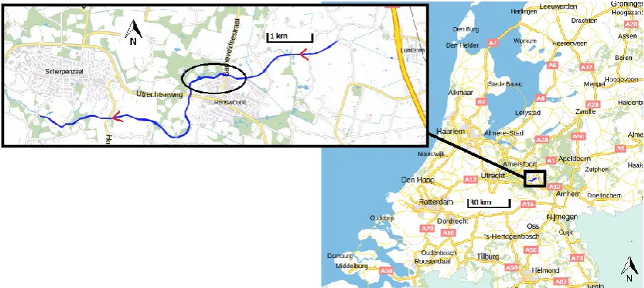
(14) Figure 3: Plan view showing the stream restoration measures performed for the course Wittenoord-Beekweide in the Lunterse beek (background photo gives the 2010 situation) In Figure 3, the course of the stream after re-meandering is shown in blue. The old straight course, as present in 2010, is shown in the background photo. It becomes clear that the course has changed significantly in the upstream section and little in the downstream section. Re-profiling, not shown in Figure 3, was performed at the same locations where re-meandering was applied. The four brown squares mark the locations where LWD is brought into the stream. The five pools that were constructed in the stream are marked by a blue circle. The two red hexagons mark the locations where the fish passage (right hexagon) and the boat ramp (left hexagon) were removed. Finally the green triangle on the very right marks the location where the weir between the Fliertse and Lunterse beek was replaced, while the green triangle in the middle marks the location where the weir Barneveldsestraat was set to a minimum level.. 2.3. The Tungelroyse beek. The Tungelroyse beek is part of the water system that is managed by water board Peel and Maasvallei. This is a water board that manages the secondary water systems in the Northern and central parts of the Limburg province, the most Southern province in the Netherlands. The location of the Tungelroyse beek is shown in Figure 4.. Figure 4: Location of the Tungelroyse beek (HKV Lijn in Water B.V., 2016) with the black circle indicating the case study area and the red arrows the flow direction 14.

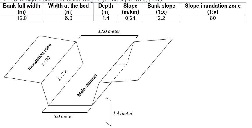
(15) Stream restoration in the Tungelroyse beek started in the headwaters of the stream in 1998, while the restoration of the middle and lower reaches started in 2005 (Coenen, 2011). Restoration was finalised in October 2011 (Waterschap Peel en Maasvallei, 2011). During the stream restoration projects, 90% of the 30 km long stream was restored (Coenen, 2011). The restoration that will be modelled in this study is the restoration project named “Tungelroyse beek Traject B”, which has a length of around 3.8 km (Pahlplatz & Droesen, 2003). The reasons for stream restoration of the Tungelroyse beek were twofold. To start with, the stream had a specific ecological function for fish, while water and sediment quality scored insufficient in the WFD. With a part of the stream being “Ecologisch Herstelproject” and an insufficient score on fish and macro fauna in the WFD, restoration was necessary in the vision of the water board. On the other hand, the bad sediment quality and the lack of natural morphology were seen as bottlenecks that had to be restored anyway (Coenen, 2011). The goal of stream restoration in the Tungelroyse beek was specified as: coherent development of morphology and ecology such that the system recovers with a focus on stream velocities and the development of possible recreation for residents in the area (Coenen, 2011). The stream restoration in the Tungelroyse beek was a re-meandering project (STOWA, 2012). The design dimensions of the Tungelroyse beek are presented in Table 3 and shown in Figure 5. Table 3: Design dimensions for the Tungelroyse beek (STOWA, 2012) Bank full width Width at the bed Depth Slope Bank slope (m) (m) (m) (m/km) (1:x) 12.0 6.0 1.4 0.24 2.2. Slope inundation zone (1:x) 80. Figure 5: Design dimensions for the Tungelroyse beek In Table 4 the discharge and water level characteristics for the Tungelroyse beek after restoration are presented. The water levels were measured between May 2011 and May 2012, while the discharge was determined based upon a theoretical relationship between water level and discharge (STOWA, 2012). Table 4: Discharge and water level characteristics Tungelroyse beek after stream restoration (STOWA, 2012) Average Daily average yearly Exceedance frequency Design discharge peak discharge inundation zone inundation time (m3/s) (m3/s) (days/year) (days/year) 1.01 5.05 6 0 Table 4 shows that the average and peak daily average discharge of the Tungelroyse beek are small. The average discharge is higher than for the Lunterse beek, while the peak daily average discharge is lower. Besides that, the exceedance frequency of the inundation zone is higher than designed, just like for the Lunterse beek. For the stream restoration project “Tungelroyse beek Traject B”, the following measures were implemented (Verlinden, 2007):   . . Re-meandering over a large part of the stream (this was done actively by digging the new course) Natural redesign of a broad area on both sides of the stream. This was performed for the entire study area, including the removal and planting of trees and bank vegetation Re-profiling of the stream in which the bed level is raised between 0 and 45 cm over the entire course and the bottom of the main channel is narrowed from 4 to 3.5 m. Also the slopes of the banks were made more steep at some locations and more gentle at others Removal of the weir named “Tun6” 15.

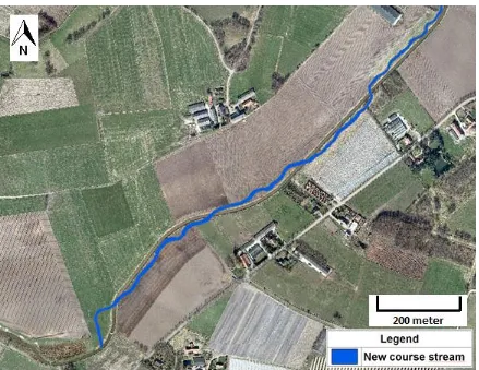
(16) The locations of these measures for the “Tungelroyse beek Traject B” course are shown in Figure 6 for the downstream section (flow from Southwest to Northeast) and in Figure 7 for the upstream section of the study area (flow from Southwest to Northeast).. Figure 6: Measures implemented in the “Tungelroyse beek Traject B” course in the downstream section (background photo shows the 2009 situation). Figure 7: Measures implemented in the “Tungelroyse beek Traject B” course in the upstream section (background photo shows the 2009 situation) Figure 6 clearly shows the new course for the downstream section of the Tungelroyse beek, with the 2009 situation as background photo. In 2009 the stream was still straight. The green triangle shows the location where the weir named “Tun 6” was removed. The new course of the Tungelroyse beek in the upstream section of Traject B is shown in Figure 7. The background photo shows the nearly straight stream as present in the 2009 situation. As can be seen, the course of the stream changed significantly due to re-meandering. 16.

(17) 3. Methodology: model set-up This chapter explains which methods are used to set-up the models. Section 3.1 explains the general methodology that is used to provide an answer to the research questions. In section 3.2 the different discharge scenarios that will be used for the model simulations are shown. Besides that, the validation locations are presented and the Q-h relationships that are fitted for these locations are shown. Section 3.3 gives a description of the structures that are relevant for the flow characteristics in both study areas. The set-up of the Sobek model for the Lunterse beek is shown in section 3.4. Section 3.5 shows how the Delft3D FM model for the Lunterse beek was set-up, while section 3.6 describes the model set-up of the Delft3D FM model for the Tungelroyse beek. Take note that no Sobek model was set-up for the Tungelroyse beek.. 3.1. General. To provide an answer to the research questions, two software packages will be used for the set-up of the models. The first is the Sobek Advanced Version 2.13.002, later referred to as Sobek, that will be used to create a onedimensional model of the Lunterse beek. The second software package is Delft3D Flexible Mesh 2016 HM, hereafter called Delft3D FM. This software will be used to set-up a two-dimensional model for both the Lunterse beek and the Tungelroyse beek. For the hydraulic comparison between the Sobek, Delft3D FM model and monitored hydraulics, a case study of the Lunterse beek will be performed. Multiple stationary discharge scenarios will be used as model forcing. The simulations will be used to compare water level output of the models to each other and to monitored water levels. The Sobek model will be based upon an already existing model that is in use with water board Vallei and Veluwe, while the Delft3D FM model will be built from scratch. Water level output of the Delft3D FM model for the Tungelroyse beek will only be compared to monitored water levels. Stationary discharge scenarios will be used as forcing for this model. The ability of the Delft3D FM model to forecast developments in morphology will be investigated for both the Lunterse and Tungelroyse beek. The main focus will be on the Lunterse beek though, since quantitative validation data is available for this stream. For the Tungelroyse beek, aerial images will be used for validation purposes. Morphological forecasts will be solely based upon hydraulic model output. For both streams locations where transport might occur will be identified using the Shields and critical Shields parameters as indicators. Besides that, flow velocity and flow direction maps will be made. Those will be compared to monitored morphological developments. For the Lunterse beek additional morphological forecasts will be made based upon flow velocity gradients. These forecasts will also be compared to monitored developments in morphology for the Lunterse beek. For the Tungelroyse beek a qualitative comparison will be performed using aerial images that show the planform development between 2012 and 2015. For both streams only a part of the study area will be used for validation of the forecasts, since validation data is lacking for the other locations. Developments in vegetation will be forecasted for both streams by using hydraulic model output of the Delft3D FM models. The forecasts will be based upon flow velocity and water depth output of the models. More vegetation is expected if flow velocities are low and less vegetation is expected if flow velocities are high (see section 4.2). For the Lunterse beek, these forecasts will be compared with developments in vegetation seen on a high resolution aerial photo. For the Tungelroyse beek the comparison will be performed using the Normalized Difference Vegetation Index (NDVI). The NDVI gives an indication for the amount of vegetation present at certain locations.. 3.2. Discharge scenarios, Q-h relations and validation locations. In this section a description is given of the discharge scenarios that will be used in the model runs for both the Lunterse beek in section 3.2.1 and for the Tungelroyse beek in section 3.2.2. Besides that, the fitted Q-h relations and the validation locations for both streams will be shown.. 3.2.1 Lunterse beek For the Lunterse beek the period for which the models will be set-up is immediately after stream restoration. Restoration of the stream was completed in November 2011. Bed level measurements were performed after stream restoration in February 2012 by Meet B.V. (2012). This data will be used to set-up a geometry for both the Sobek and Delft3D FM model. The period for which the model is supposed to be representative is therefore 01-12-2011 till 15-02-2012. Multiple locations are present in the study area that are important for the set-up and validation of the models. These locations are presented in Figure 8 and their characteristics are shown in Table 5.. 17.

(18) Figure 8:Model boundaries and locations for model validation of the Lunterse beek (Google Maps) Table 5: Boundaries and validation locations for the Lunterse beek Location Type of measurement Name Upstream boundary Nothing Groot Abbelaar downstream Validation location 1 Water levels WL2 Validation location 2 Water levels and discharge Barneveldsestraat upstream Validation location 3 Water levels and discharge Barneveldsestraat downstream Downstream boundary Water levels Utrechtseweg As becomes clear from Table 5, no discharge measurements were performed at the upstream boundary. Therefore the discharge measurements performed at the Barneveldsestraat will be used as model forcing. This can be done since inflow between the upstream boundary and the discharge measurement station of the Barneveldsestraat, through run-off and groundwater flow, is minimal compared to the discharge of the stream. Besides that, only stationary discharge scenarios will be used in the simulations and therefore changes in discharge shape between the upstream boundary and the Barneveldsestraat are not important for the model simulations. At the downstream boundary a weir is present. Therefore, the water level measurements performed just upstream of this weir will be used as boundary condition for the model while the weir will be neglected in the model simulations. For the validation of the model output, the water levels measured at locations 1, 2 and 3 will be used. For the model simulations, multiple model runs will be performed using stationary discharge scenarios. To start with, 5 discharge scenarios were selected that are important from a hydrological point of view:     . The discharge that is exceeded 0,01 days per year (extreme peak, T100) The discharge that is exceeded 0,1 days per year (design norm rural area, T10) The discharge that is exceeded 1 day per year (design discharge, T1) The discharge that is exceeded 20 days per year (high spring discharge, T0.05) The discharge that is exceeded 200 days per year (average summer discharge, T0.005). To match discharge values to the lower range scenarios (T1, T0.05 and T0.005), a measurement series collected by water board Vallei & Veluwe between 01-12-2011 and 03-03-2016 at the Barneveldsestraat measurement station will be used. The reasoning behind this is that after restoration of the stream, discharge characteristics were altered since the weir Barneveldsestraat was set to a minimum level. Therefore data collected before 01-12-2011 cannot be used. Besides that, discharge measurements at the Barneveldsestraat only started in 2011. For the higher range scenarios (T10 and T100), information from the report: Hermeandering Lunterse Beek: Effectenberekeningen (Versteeg et al., 2010) was used. The resulting match between the discharge scenarios and the discharge values is presented in Table 6. Table 6: Discharges for different scenarios Discharge scenario Discharge (m3/s) Average summer discharge (T0.005) 0.192 High spring discharge (T0.05) 1.264 Design discharge (T1) 3.61 Design norm rural area (T10) 7.40 Extreme peak (T100) 10.06 Beside these important discharge scenarios from a hydrological point of view, 11 other discharge scenarios were selected for validation specifically. Since for these scenarios the period directly after stream restoration was assumed, data collected between 01-12-2011 and 15-02-2012 was analysed to conclude that these 11 scenarios need to range from 0.5 m3/s up to 5.5 m3/s, with 0.5 m3/s increments to describe a range of discharge values that covers the range of the measurements, as can be seen from Figure 9. 18.

(19) Figure 9: Discharge series for the Lunterse beek, collected at the Barneveldsestraat measurement station between 01-12-2011 and 15-02-2012 Data collected between 01-12-2011 and 15-02-2012 was used to derive Q-h relationships for the validation locations and the downstream boundary. The MatLab curve fitting tool was used to fit the Q-h relationships through the measurements. The decisions made during the fitting process as well as the fit characteristics are shown in Appendix A. The fitted Q-h relationships are presented in Figure 10 including the measured water levels. The boundary conditions based upon the Q-h relation at the Utrechtseweg are shown in Table 7. For the design norm rural area (T10) and peak discharge (T100) events, a different Q-h relation was used than the one presented here. This Q-h relation can be found in Appendix A also. Table 7: Boundary conditions for the models of the Lunterse beek Model run Upstream discharge Downstream water level (m3/s) (m) 1 0.5 4.91 2 1.0 4.96 3 1.5 5.04 4 2.0 5.12 5 2.5 5.22 6 3.0 5.32 7 3.5 5.42 8 4.0 5.50 9 4.5 5.57 10 5.0 5.62 11 5.5 5.65 12 0.192 4.91 13 1.264 5.00 14 3.61 5.44 15 7.40 5.99 16 10.06 6.46. 19. Remarks Model validation Model validation Model validation Model validation Model validation Model validation Model validation Model validation Model validation Model validation Model validation Average summer discharge (T0.005) High spring discharge (T0.05) Design discharge (T1) Design norm rural area (T10) Peak discharge (T100).

(20) Figure 10: Fitted Q-h relations for the Lunterse beek with their locations In Figure 10 a hysteresis effect becomes visible. This means that the water levels after the peak are higher than the water levels before the peak for equal discharges, due to a time-lag between changing flow conditions and changing bed roughness (Paarlberg et al., 2010). Since stationary discharge scenarios are used in this study, this effect is not taken into account in the simulations. However, for the fitting of the Q-h relations this effect is accounted for, meaning that uncertainty is introduced for the validation of water levels.. 3.2.2 Tungelroyse beek The period directly after stream restoration is of interest for the model set-up of the Tungelroyse beek. Restoration of the section of interest was finalised in March 2011 (Waterschap Peel en Maasvallei, 2011). However, since the section of interest is quite long, bed level measurements were performed after restoration in the period between 2010 and 2011 (Menten & Strigencz, 2012). These bed level measurements will be used for the set-up of a geometry in the Delft3D FM model. The modelling period will therefore be 2010-2011. For the Tungelroyse beek, 3 locations are important for model set-up and validation of model results. These locations are shown in Figure 11 and their characteristics are presented in Table 8.. 20.

(21) Figure 11: Model boundaries and validation location for the Tungelroyse beek (Google Maps) Table 8: Boundaries and validation location for the Tungelroyse beek Location Type of measurement Name Upstream boundary Nothing Wisbroek Validation point Water level Castertbrug Downstream boundary Water level OTUNG17 From Table 8 it becomes clear that no discharge measurements were performed at the upstream boundary. Besides that, at the validation location and the downstream boundary no discharge measurements were performed either. Therefore the upstream discharge needs to be derived from measurements performed outside of the study area. A schematic overview of the available data is given in Appendix B. Measurement location OTUNG13, located almost 7.5 km downstream of the upstream boundary Wisbroek, will be used to derive the discharge for the upstream boundary. To start with, it has to be noted that discharge measurements at location OTUNG13 are affected by inflow from another stream, namely the Leukerbeek. Therefore, the discharge measured at this location will be higher than the discharge expected at Wisbroek, the upstream boundary of the model. The catchment areas of the Tungelroyse beek and Leukerbeek were used, in combination with knowledge from water board Peel and Maasvallei, to determine that the discharge ratio between the Leukerbeek and the Tungelroyse beek is around 1:2 at their confluence. Besides inflow from the Leukerbeek, the discharge measurement at OTUNG13, further downstream of the study area, will be higher by extra inflow through groundwater flow and run-off. The catchment area of the Tungelroyse beek indicates that the drainage area in-between Wisbroek and OTUNG13 is around 25% of the total catchment area. The normative discharge map, that gives an indication for the peak yearly discharge in the whole stream, shows that the peak yearly discharge in the section Wisbroek is around 80% of the peak yearly discharge just before confluence of the Leukerbeek and Tungelroyse beek. It is therefore assumed that the discharge at Wisbroek will be 20% lower than the discharge measured at OTUNG13 due to run-off and groundwater inflow. A combination of the 1:2 discharge ratio between the Leukerbeek and Tungelroyse beek and 25% extra inflow through run-off and groundwater flow gives an indication of 8/15 for the discharge measured at OTUNG13 to occur at Wisbroek. Using this factor to relate discharge measurements increases model uncertainty, since variations in discharge between the Leukerbeek and Tungelroyse beek will be present over time that are not accounted for. Besides that, the inflow through run-off and groundwater flow will not be constant over time. However, since other measurements are not available this is the best possible guess that can be used. An advantage is that only stationary discharge scenarios will be used, making that changes in discharge shape can be ignored. 21.

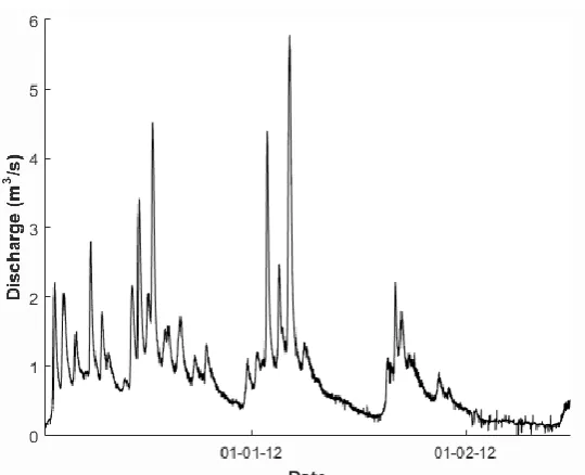
(22) For the Tungelroyse beek 5 important discharge scenarios from a hydrological point of view will be used, just like for the Lunterse beek:     . The discharge that is exceeded 0,01 days per year (extreme peak, T100) The discharge that is exceeded 0,1 days per year (design norm rural area, T10) The discharge that is exceeded 1 day per year (design discharge, T1) The discharge that is exceeded 20 days per year (high spring discharge, T0.05) The discharge that is exceeded 200 days per year (average summer discharge, T0.005). For the study area of the Tungelroyse beek, 3 obviously different periods could be distinguished in the available data. The first period was before stream restoration with data available from 31-03-2009 till 08-03-2011. The second period was after stream restoration with data available from 08-03-2011 till 16-08-2013. The third period was after stream restoration also, but with a large change in catchment area of the Leukerbeek. Data for the third period ranges from 16-08-2013 till 19-06-2016. To determine the discharge for the lower discharge scenarios (T1, T0.05 and T0.005), data collected in the second period was used. A plot of the daily discharge and water level data collected in the second period for the downstream boundary and validation location is shown in Figure 12. For the higher discharge scenarios (T100 and T10), the discharge belonging to those scenarios was based upon the 10 highest discharge events only. Extrapolation of the fitted curve was performed to determine the discharge for these extreme scenarios.. Figure 12: Relation between daily discharge and daily water level measurements at the validation location and downstream boundary for the Tungelroyse beek in the period 08-03-2011 till 16-08-2013 As becomes clear from Figure 12, very clear relations between discharge and water levels are absent. Part of this can be explained by the assumption that the discharge ratio between the Leukerbeek and Tungelroyse beek is fixed at 1:2, which will not be the case in reality. Changes in this discharge ratio will cause a horizontal shift in the measurements. A vertical shift in measurements is likely caused by the delay that occurs in reality between the upstream boundary and the OTUNG13 measurement station 7.5 km downstream. This is not accounted for in this study, but will cause a mismatch between measured discharge and measured water levels, even if daily measurements are used (take note that if the water velocity is 0.2 m/s the delay in discharge will already exceed 10 hours). Another part of the variation might be caused by differences in bed roughness for different periods though. To see how much roughness changes affect the results, data was split for every month. These monthly relationships are presented in Figure 13 for the months December until March. As becomes clear from Figure 13, when monthly Q-h relations are used instead of yearly ones, much less data is available. However, it also shows that a better relationship is present between monitored discharge and water level. It was therefore chosen to use a monthly Q-h relation for the stationary discharge simulations. The month of December was selected, because the highest range in discharge was present for this month. It can therefore be concluded that the modelled period is December 2011. From the measurements in December 2011, it becomes clear that 6 other stationary discharge scenarios should be sufficient for validation of the Tungelroyse beek model. These scenarios should range up to 3.0 m3/s with 0.5 m3/s increments. The MatLab curve fitting tool was used to fit the Q-h relationships through the measurements. The decisions made during the fitting process as well as the fit characteristics are shown in Appendix C. The fitted Q-h relationships, including the measured water levels are presented in Figure 14. The boundary conditions based upon the Q-h relation at OTUNG17 are presented in Table 9.. 22.

(23) Figure 13: Relations between upstream discharge and water levels for the Tungelroyse beek at the downstream boundary and at validation location Castertbrug for the months December till March Table 9: Boundary conditions for the Tungelroyse beek models Model run Discharge (m3/s) Water level (m +NAP) 1 0.5 27.04 2 1.0 27.22 3 1.5 27.40 4 2.0 27.56 5 2.5 27.72 6 3.0 27.88 7 0.322 26.98 8 1.205 27.29 9 2.566 27.75 10 4.2 28.22 11 6.2 28.58. 23. Remarks Model validation Model validation Model validation Model validation Model validation Model validation Average summer discharge (T0.005) High spring discharge (T0.05) Design discharge (T1) Design norm rural area (T10) Peak discharge (T100).

(24) Figure 14: Fitted Q-h relations for the Tungelroyse beek Uncertainties were introduced in the process performed to obtain boundary conditions and validation data for the models. The main source of uncertainty will likely be caused by the transformation performed to obtain the discharge at the upstream location. This will affect Q-h relations for the downstream boundary and validation location.. 3.3. Structures. This section gives a description of the structures that are relevant for the flow characteristics of both the Lunterse and Tungelroyse beek. Section 3.3.1 gives a description for the Lunterse beek and section 3.3.2 for the Tungelroyse beek.. 3.3.1. Lunterse beek. In the Lunterse beek multiple structures are present that alter flow characteristics. Both hard structures and soft structures are present in the stream. The hard structures are the bridge “Barneveldsestraat” and the weir “Barneveldsestraat”. The soft structures are 4 packages of LWD that are placed in the Lunterse beek as part of the restoration project. The locations and images of these structures are shown in Figure 15, while the dimensions are presented in Table 10. As noted in section 3.2.1 a weir is also present at the downstream boundary, but since the water levels just upstream of this weir are used, this hard structure is neglected in this analysis. Table 10: Dimensions of the structures that affect water flow in the Lunterse beek Name structure Bridge Weir LWD “Barneveldsestraat” “Barneveldsestraat” 1 Width (m) 12.0 7.7 12.0 Height (m) 2.51 (-) (-) Crest level (m +NAP) (-) 4.59 (-) Length (m) 13 (-) 22.9 Area (m2) (-) (-) 228.0 Thickness bridge deck (m) 0.5 (-) (-) Top level bridge (m +NAP) 7.43 (-) (-) Manning roughness (s/m1/3) 0.014291 (-) 0.1. 1. The Manning roughness was based upon the Sobek model 24. LWD 2 8.2 (-) (-) 16.1 120.7 (-) (-) 0.1. LWD 3 10.8 (-) (-) 20.6 175.7 (-) (-) 0.1. LWD 4 7.8 (-) (-) 20.3 137.5 (-) (-) 0,1.

(25) Figure 15: Relevant structures for water flow in the Lunterse beek study area with: 1) Bridge "Barneveldsestraat" 2) Weir "Barneveldsestraat" 3) First LWD package 4) Second LWD package 5) Third LWD package 6) Fourth LWD package. 3.3.2 Tungelroyse beek In the study area of the Tungelroyse beek 2 hard structures are present that affect flow processes. The first structure is the bridge “Wisbroek” and the second structure is the “Castertbrug”. The locations of these bridges along with an image of them is shown in Figure 16. The dimensions are presented in Table 11.. Figure 16: Location of structures that are relevant for water flow in the Tungelroyse beek with: 1) Bridge “Wisbroek” 2) “Castertbrug” Table 11: Dimensions of the relevant structures for water flow in the Tungelroyse beek Name structure Bridge “Wisbroek” “Casterbrug” Width (m) 4.4 5.5 Height (m) 1.8 2.0 Length (m) 2.7 5.25 Thickness bridge deck (m) 0.5 0.7 Top level bridge (m +NAP) 29.8 29.3 Manning roughness (s/m1/3) 0.013332 0.013332 2. (Hager, 2010) 25.

(26) 3.4. Sobek model Lunterse beek. The Sobek model as used by water board Vallei and Veluwe was used as a starting point for the set-up of a Sobek model for the Lunterse beek. This model was made by HKV Lijn in Water as part of the “Nationaal Bestuursakkoord Water” (NBW) (Graaff & Jungermann, 2014). This model includes all streams that are managed by water board Vallei and Veluwe. For this study it is important to note that the model was set-up without taking into account the stream restoration that took place at the Wittenoord-Beekweide course. This means the model needs to be adjusted to describe the situation after restoration of the stream correctly. Six adjustments were performed on the initial model. This was done at water board Vallei and Veluwe: 1. All sections, including all the structures outside of the study area (as described in section 2.2) were deleted and flow boundaries were added to the model at the locations of the up- and downstream boundaries of the Wittenoord-Beekweide course. 2. Bed levels of the stream were altered so that those agreed with the period that is modelled for the Lunterse beek (01-12-2011 till 15-02-2012). To alter the geometry, all the cross sections in the initial model were deleted and the measurements performed by Meet B.V. (2012) in February 2012 were imported in the Sobek model using the IRIStoSobek tool obtained from water board Vallei and Veluwe. 3. After modifying the study area extent and the bed levels, the settings of the weir Barneveldsestraat were changed. As explained in section 2.2 the weir was lowered to its minimal level during the restoration project. 4. The length of the flow links was changed in order to represent the new meandering length of the main channel. 5. Monitoring stations were added at the locations where validation of water levels need to take place (see section 3.2.1). 6. Bed roughness values were changed to represent the period directly after stream restoration. This resulted in a new model geometry that is shown in Figure 17.. Figure 17: Final model geometry for the Sobek model of the Lunterse beek The sixth adjustment performed in the model was to determine the bed roughness for the period directly after stream restoration. The bed roughness was specified for the Sobek model using the Manning roughness coefficient. This decision was made, because research showed that the Manning roughness parameter gives good results for vegetation that has a relatively high water depth on top of it (Huthoff, 2014). For the Lunterse beek this is likely to be the case in most of the study area, since a winter situation is modelled in which vegetation will be scarcely present. The locations where this is not likely to be the case are the locations where LWD was placed during restoration. The effect of using the Chézy roughness parameter (that gives better results when vegetation is relatively high compared to water levels (Huthoff, 2014)) instead of Manning in this section will be analysed in Appendix D. The Manning roughness values for the Sobek simulations were determined using the Cowan method (Cowan, 1956). The Cowan method makes use of the formula listed below to take two-dimensional effects into consideration when setting up a one-dimensional model:. 𝑀𝑎𝑛𝑛𝑖𝑛𝑔′ 𝑠 𝑛 = (𝑛𝑏 + 𝑛1 + 𝑛2 + 𝑛3 + 𝑛4 )𝑚 The two-dimensional effects described by the different parameters are shown in Table 12. Take note that Cowan (1956) makes a distinction between the main channel and the floodplain when determining the roughness parameters.. 26.

(27) Table 12: The two-dimensional effects described by the different parameters in the Cowan method Parameter Explanation main channel Explanation floodplain nb Channel material Floodplain material n1 Degree of irregularity Degree of irregularity n2 Variation in channel cross-section Variation in floodplain cross-section n3 Effect of obstructions Effect of obstructions n4 Amount of vegetation Amount of vegetation m Degree of channel meandering Floodplain meander Since the stream shows considerable variations with respect to the different parameters listed in Table 12, three different sections were distinguished. Section one is the most upstream section and has been actively restored by re-meandering. This section is highlighted in Figure 18.. Figure 18: First section for the Sobek schematization regarding bed roughness (photo 2012) Section two is also a part that was actively restored by re-meandering, however this section is clearly different from the first section since LWD was placed in the stream. Section 2 is presented in Figure 19. The locations where LWD is placed are marked with red circles.. Figure 19: Second section for Sobek schematization regarding bed roughness (photo 2012) The third and most downstream section that was distinguished is different from the first two sections since it was not actively restored. The straight planform shape of the stream was maintained in section three as can be seen in Figure 20.. 27.

(28) Figure 20: Third section for Sobek schematization regarding bed roughness (photo 2012) Besides differences in the alongshore direction of the stream, cross-shore differences were found. To start with, there is a difference in roughness between the main channel and the floodplains of the stream. This difference is also recognized by Cowan (1956). Both sections use the basic formula, but there is a difference in the parameter values and descriptions, as can be seen in Table 12. For this study a distinction was also made between the close floodplain and the distant floodplain of the stream. The close floodplain is the part that was actively restored just like the main channel, while the distant floodplain was not. Besides this, the close floodplain is designed to actively participate in discharging water when water levels exceed a certain threshold. The distant floodplains on the other hand are often formed by pasture grounds that might flood during high discharge events, but are not meant to inundate. As explained in section 3.2.1, 16 uniform discharge scenarios will be used for the model simulations with the modelled period ranging from 01-12-2011 until 15-02-2012. This means that stream restoration was just finished at that time and vegetation was still absent. The Cowan method gives a range for all parameter values. For all calculations it was chosen to use the average value for the simulations. In Appendix D, the effect of this decision is investigated. In Table 13 the parameter values that will be used in the Sobek simulations are presented. Argumentation for selecting these values is given in Appendix E. Table 13: Manning roughness values for Sobek simulations with uniform discharge scenarios Section Channel type nb n1 n2 n3 n4 m nFinal 1 Main channel 0.024 0.003 0.003 0.002 0.006 1 0.038 1 Close floodplain 0.024 0.008 0 0.002 0.006 1 0.040 1 Distant floodplain 0.024 0.008 0 0.025 0.0375 1 0.095 2 Main channel 0.024 0.003 0.003 0.025 0.006 1.15 0.070 2 Close floodplain 0.024 0.008 0 0.002 0.006 1 0.040 2 Distant floodplain 0.024 0.003 0 0.01 0.0375 1 0.075 3 Main channel 0.024 0.008 0 0.002 0.006 1 0.040 3 Close floodplain 0.024 0.003 0 0.002 0.006 1 0.035 3 Distant floodplain 0.024 0.003 0 0.01 0.0375 1 0.075 It may appear strange that in section 2 the roughness in the main channel exceeds the close floodplain roughness and is relatively close to the distant floodplain roughness. However, this is solely caused by the LWD that is present in the main channel as can be seen from parameter n 3.. 28.

(29) 3.5. Delft3D FM model Lunterse beek. In this section a description is given of how the Delft3D FM model for the Lunterse beek was set-up. The study area for the Lunterse beek was presented in section 2.2. For the Delft3D FM model this exact area is used to set-up the model. The lateral extent of the study area was harder to determine, since there is no levee or physical barrier present for the Lunterse beek floodplains. Therefore AHN2 data (Publieke Dienstverlening Op de Kaart, 2015) was used to determine the channel boundaries. An estimate of the maximum water level for the stream was made with an additional height of 0.3 m. This resulted in an extent of the study area as presented in Figure 21. To give more insight in how this corresponds to the study area of the Sobek model, the cross-section measurements (Meet B.V., 2012) that define the extent of the Sobek model are also shown in Figure 21.. Figure 21: Study area of the Delft3D FM model (red line) for the Lunterse beek with the cross-sectional measurement locations in purple (Meet B.V., 2012) (photo 2012) Figure 21 shows that the study area of the Delft3D FM model is larger than the study area of the Sobek model. A check for the Delft3D FM model showed that the study area was chosen large enough for the discharge scenarios that are used in this study. Water will remain within the study area specified in Figure 21 for all discharge scenarios. For the Sobek model it was found that the study area was not large enough in the upstream section for discharges exceeding 5.0 m3/s (for the 1st to 5th cross-section in the study area). In the Sobek model, water will stay within the model since a vertical wall will be assumed at the outer boundaries of each cross-section. It has to be taken into account though that simulated hydraulics will be slightly affected in this section. Simulated water levels will likely be higher as are flow velocities (due to the absence of roughness in this area). After defining the study area, a grid was set-up for calculations in the Delft3D FM software. For the main channel, a curvilinear grid was set-up with an average cell size around 0.4 by 1.0 m in lateral and flow direction respectively. This makes that the main channel has 18 cells in lateral direction and around 2000 cells along the stream. For the floodplains a triangular grid was created. Close to the main channel cell size lies around 1 x 1 x 1 m. Figure 22 shows part of the grid in which the main channel (curvilinear grid) is already connected to the floodplains (non curvilinear grid).. Figure 22: Part of the grid in the Delft3D FM model (Lunterse beek) showing the main channel and the floodplain 29.

(30) Towards the outer edges of the floodplains, the cell size of the grid increases gradually. At the most outward boundaries of the floodplains the cell size varies between 4 x 4 x 4 meter up to 10 x 10 x 10 meter, depending on how far the location is situated from the main channel. After generating a grid, the bathymetry of the main channel was created. For this, the same cross-sectional measurements were used as for the Sobek model (Meet B.V., 2012). However, since a complete bathymetry is required for the Delft3D FM model an interpolation of the data was needed. For this interpolation, the tool Surfis2D (RIZA Rijkswaterstaat, 2004) was used. This tool was developed by Rijkswaterstaat and is specifically suited to interpolate river cross-section measurements to a complete bathymetry while taking into account the meandering shape of the waterway. The sensitivity for this interpolation tool is tested in Appendix F. It was found that the bathymetry obtained with the Surfis2D interpolation tool is highly dependent upon the amount of cross-sectional bed level measurements used as input. For this specific test is was found that the bathymetry is on average higher if less cross-sectional bed level measurements are used. The measurements performed by Meet B.V. (2012) were also used to create a bathymetry for the floodplains where possible. At locations where measurements were missing, AHN2 (Publieke Dienstverlening Op de Kaart, 2015) data was used. This made it possible to create a bathymetry that was nearly covering the entire study area. An analyses in differences between AHN2 data and measurements is presented in Appendix G, since AHN2 data was measured in 2010 while the modelling period is the winter of 2011/2012. Comparison between the measured bed levels and AHN2 data showed that on average the bottom level was 0.27 m higher for the AHN2 measurements. This will result in higher simulated water levels if flow occurs in these areas. For the locations where both AHN2 measurements and measurements performed by Meet B.V. (2012) were missing, the below given assumptions were made:   . Buildings: bed level height 12 m +NAP (means a height of around 7 m for all buildings) Waters that are not part of the Lunterse beek: a water depth of 0.5 m relative to surroundings Other areas: equal height to surroundings. This resulted in a complete bathymetry for the Delft3D FM model that is presented in Figure 23.. Figure 23: Bathymetry for the Delft3D FM model of the Lunterse beek To define the bed roughness in Delft3D FM, a spatially varying roughness was used over the entire grid. The roughness was defined using the Manning roughness parameter as was used in the Sobek model. The roughness values were determined based upon typical characteristics of the different parts in the study area. The different types of area that were distinguished for the Lunterse beek are presented in Table 14. Table 14: Different characteristic areas in the Lunterse beek study area Type Characteristics Main channel Sandy bottom Floodplain close to main channel Sandy bottom Pasture Grass Large Woody Debris Trees Roads Asphalt Houses Bricks Forest Trees Garden Diversified. 30.

(31) For the different areas, roughness values were selected using the “Cultuurtechnisch Vademecum”, in which a range of km roughness values is specified. These values were converted to Manning roughness values using the formula specified below (Ribberink & Hulscher, 2012): 𝑅1/6 (Eq. 1) 𝐶 = 𝑅1/6 ∗ 𝑘𝑚 = 𝑛 From this it follows that: 1 𝑛= 𝑘𝑚. (Eq. 2). The Manning roughness values that will be used in the simulations with the Delft3D FM model are presented in Table 15 and Figure 24. Besides that, Table 15 specifies the range for these roughness values. The range is determined by the upper and lower limits of the selected roughness categories for the different vegetation types. The motivation for using these values is given in appendix H. Table 15: Manning roughness values (n) for the different area types in the Delft3D FM model for the Lunterse beek Type nlower nupper nselected Main channel 0.022 0.05 0.033 Floodplain close to main channel 0.022 0.05 0.033 Pasture 0.05 0.2 0.1 Large Woody Debris 0.075 0.125 0.1 Paved area 0.029 0.067 0.05 Houses 1 1 1 Forest 0.1 0.5 0.2 Garden 0.05 0.2 0.1. Figure 24: Spatially varying roughness in the Delft3D FM model for the Lunterse beek. 3.6. Delft3D FM model Tungelroyse beek. This section describes how the Delft3D FM model for the Tungelroyse beek was set-up. The study area for the Tungelroyse beek was presented in section 2.3. For the Delft3D FM model this exact area is used to set-up the model. The lateral extent of the study area was determined based on AHN2 data (Publieke Dienstverlening Op de Kaart, 2015), since no levee or physical barrier is present for the floodplains of the Tungelroyse beek. By estimating the maximal water level in the study area and a margin of 0.3 m, the extent of the study area as presented in Figure 25 was obtained.. 31.

No results found