Change in 3d periarticular bone density after Knee Joint Distraction or High Tibial Osteotomy in the treatment of osteoarthritis

(1)

Bachelor Thesis Technical Medicine

Multidisciplinary Assignment

CHANGE IN 3D PERIARTICULAR BONE DENSITY AFTER

KNEE JOINT DISTRACTION OR HIGH TIBIAL OSTEOTOMY

IN THE TREATMENT OF OSTEOARTHRITIS

Authors:

N. A. Coorens s1452789

C. J. Ensink s1245449

J. W. van der Graaf s1760599

B. Schippers s1448404

Supervisors:

Prof. Dr. C. H. Slump

MSc. N. J. Besselink

Dr. S. C. Mastbergen

Dr. P. de Jong

(2)

Abstract

Background: Osteoarthritis (OA) is a degenerative joint disease, associated with both cartilage

and periarticular bone change. High Tibial Osteotomy (HTO) is a generally considered method for prolonging the time before a total knee replacement is necessary and to reduce the pain

in patients suffering from OA. A relatively new technique is Knee Joint Distraction (KJD). Although there is evidence for an improvement of cartilage after KJD, changes in periarticular

bone have not yet been investigated.

Objective: The main goal of this research is to determine the difference in quality of periarticular

bone of the tibia before and two years after treatment with KJD or HTO using 3D Computed Tomogrophy (CT).

Methods: Coronal CT images were obtained from two previous conducted studies, a total of 23 patients (mean age 51±7 years; 15 males, 10 KJD) were included. Changes in bone density

are related to changes in intensity, measured in Hounsfield Units (HU). In the assessment of the periarticular bone quality, a distinction was made between subchondral and trabecular bone,

by calculating intensities in five different layers to a depth of 5 mm beneath the joint surface of the tibia. Bone quality was expressed in mean absolute deviation (MAD) and mean intensity.

Results: Mean intensities seem to be decreased at two year follow up compared to baseline, but these differences were statistically insignificant in both HTO and KJD. Interestingly, in the case

of KJD, the MAD of the intensities in all layers of the lateral compartment and some layers of the medial and other compartments, were significantly decreased.

Conclusions: The results suggest that periarticular bone density neutralizes. This was

(3)

Preface

Before you lies the thesis that we made as a completion of the bachelor and premaster in Technical Medicine at the University of Twente. It is a reflection of the competences and an opportunity to show the knowledge we acquired during the past years.

We have gained more experience in using software like LaTeX, SPSS and especially Matlab. We cheered and raised our hands in the air when Matlab showed us what we wanted it to show, but we execrated it when the red lines popped up for the umpteenth time.

To us, performing this research was an interesting challenge, in which we have felt delighted, as well as disheartened. But: “If the job was easy, there should be no need of the technical medical profession.” We would like to thank Cees Slump for this insight and many more he gave us dur-ing the process. Another thanks to Matti`enne van der Kamp for keeping an eye on the process and guiding our personal and professional development. Furthermore we would like to thank our supervisors from the UMC Utrecht for their supervision and contribution in this project. Special thanks to Nick Besselink, who was always available and willing to guide and support us during these ten weeks.

(4)

OA is a degenerative joint disease, which is characterized by progressive degeneration of car-tilage, subchondral sclerosis, osteophyte formation, changes in periarticular structures and joint inflammation, as shown in figure 1.[3] These changes often lead to pain, stiffness and reduced mobility of the joint. The main cause of OA is still unclear, but there is evidence that biomech-anical changes lead to damaged cartilage and bone, deteriorating the joint and inducing OA.[4] It is believed that this process is counteracted by the formation of osteophytes which try to restore mechanical load within the joint.[5]

[image:5.595.184.408.364.518.2]

Periarticular bone is composed of subchondral and trabecular bone. In OA, the formation of osteophytes and cysts can be found in the subchondral bone and trabecular bone. Subchondral bone thickness in the knee joint can vary from approximately 0.1 – 1.5 millimeter, where maxima can be seen at the central zones of the tibia and minima at the peripheral zones.[6]

Figure 1: Schematic illustration of changes in osteoarthritis.[7]

1.2 Treatments

Because OA still is an incurable disease, treatment focuses on reducing the symptoms. This is mainly done by reducing the load on the knee, physiotherapy and painkilling.[8] If these options do not improve the circumstances sufficiently, surgery could be another possibility. High Tibial Osteotomy (HTO) relieves the pressure on the affected side of the knee by correcting the angle between the femur and tibia. This procedure is usually done if the medial side of the knee is affected by OA. An HTO can be done by the medial opening wedge or the lateral closing wedge technique. With both approaches the load on the medial side decreases while the load increases on the lateral side of the knee joint. In this way, the stress on the affected side is reduced.[9]

(6)

well understood how these principles exactly work.[12] The aim of both HTO and KJD, especially in relatively young patients, is to reduce the pain and stiffness related to OA and postpone the placement of a prostatic knee, which is the final option to treat OA.[10]

[image:6.595.111.283.125.300.2]

(a) Opening wedge HTO treatment.[13] (b) KJD treatment.[14]

Figure 2: Two possible treatments for OA.

1.3 Study goal

(7)

2 Methodology

2.1 Computed Tomography

For this research, CT images were used to compose a 3D reconstruction of the tibia, so the intensity displayed by the voxels represent the bone density at a specific anatomical position. The use of CT is an advantage over the conventional bone density measurements, so called DEXA scans, because it assesses the volumetric density (mg/cm3) rather than the 2D area density (g/cm2) generated from a DEXA scan.[15]

Because the DEXA scan is only two dimensional, it calculates the mean intensity along the direction of the scan axis. For this reason, a DEXA scan would be insufficient to assess changes in bone density because the increased and decreased intensities at different locations that can be found in OA will give a mean value that is comparable to the mean intensity in healthy bone tissue. Therefore, the displayed values by use of a DEXA scan are not truly representative for the bone density. The 3D CT reconstruction can display the intensity for every different voxel in the 3D space, making it more suitable to assess changes in bone density.[16]

2.2 Subjects

Subjects were selected from two trials reviewed by the Medical Ethical Committee (MEC #11-072 and MEC #10-359). Patients were all diagnosed with severe OA of the knee and indicated for a HTO by an orthopaedic surgeon. The inclusion criteria for both trials were set as followed:[17]

– Patients with medial or lateral tibio-femoral compartmental OA considered for HTO accord-ing to regular clinical practice;

– Age<65 years;

– Radiological joint damage: Kellgren and Lawrence score >2;

– Intact knee ligaments;

– Normal range-of-motion (min. of 120° flexion);

– Normal stability;

– Body Mass Index <35.

Exclusion criteria for this research were:

– Mechanic axis-deviation (varus-valgus)<10 degrees;

– Psychological inabilities or difficult to instruct;

– Not able to undergo MRI examination (standard daily clinical practice protocol);

– Inflammatory or rheumatoid arthritis present or in history;

– Post traumatic fibrosis due to fracture of the tibial plateau;

– Bone-to-bone contact in the joint (absence of any joint space on X-ray);

– Surgical treatment of the involved knee< 6 months ago;

– Contra-lateral knee OA that needs treatment;

(8)

2.3 Data Collection

CT images of the subjects were provided by the department of Rheumatology and Clinical Im-munology, University Medical Center Utrecht, and made by a Phillips Brilliance ‘64 CT scanner. These CT images were taken prior to treatment (baseline) and at two years of follow up and were obtained in the period from July 2012 to September 2015. To process the data, as described in the following section, scans containing a coronal view of the knee joint were used. Therefore, CT data of 23 patients (mean age 51±7 years; 15 males, 10 KJD) were included.

2.4 Data Processing

In order to obtain 3D results that can be analysed to assess the quality of the periarticular bone, the data was processed through the actions written below. All processing was done with the use of Matlab R2015b. An overview of the processing steps can be found in a flowchart in appendix I. An explanatory list of certain Matlab commands can be found in appendix II.

2.4.1 Load DICOM files

The script that was used to read the DICOM files in Matlab was based on a script retrieved from Matlab Central/File Exchange.[18] Some adjustments were made to meet specific requirements. The output of the script is a volume image matrix of the loaded DICOM files.

2.4.2 Segmentation

Medical image segmentation is an important part of the data processing. Using segmentation, a region of interest, in this case bone tissue, can be extracted from surrounding tissues in medical images. Many segmentation methods exist, both automatic and semi-automatic.

(a) Segmentation based on a global threshold of 306 Hounsfield Units.

(b) Segmentation based on a local threshold ob-tained with the imrect function in Matlab.

(c) Segmentation based on a global threshold ob-tained with Otsu’s method.

[image:8.595.321.531.469.574.2]

(d) Segmentation based on a global threshold by visual assessment.

(9)

To extract bone from the surrounding tissue, techniques like global, local and Otsu’s thresholding and region growing were considered. A comparison of different segmentation methods, as can be seen in figure 3, showed minimal differences in accuracy. Global thresholding by use of one certain threshold value appeared to be the fastest and least subjective method to segment the bone tissue from the surrounding soft tissue. Therefore, segmentation was done based on one threshold value of 306 Hounsfield Units (HU). This value can separate high intensity voxels (e.g. cortical bone) from low intensity voxels (e.g. soft tissue).[19]

2.4.3 Splitting tibia and femur

In order to look at the tibial plateau, the femur had to be removed from the 3D reconstruction. Based on the assumption that both tibia and the femur are two different connected structures, the tibia and femur were labelled by the functionbwconncomp after segmentation. After the labelling of both bones, the femur was removed from the 3D image, based on the hight. In order for this method to work the tibial and femur bone cannot be connected at any location in the scan. By using the function imerode, all the edges of both bones were reduced by one pixel to minimize the chance that the tibia and femur would still be connected. This created small gaps in the images which were partially repaired using the imclose function. Scans that had the tibia and femur still connected after this adjustment were excluded from this research, which was the case in the scans of eight subjects. Apart from splitting the bones, this section of the script was also used to filter the scan. Smaller groups of pixels that were not connected to either the tibia or femur were extracted from the data.

2.4.4 Intensity and location of tibial plateau

Bone changes were tracked by five layers of each 1 mm following the bone contours, to a total depth of 5 mm from the joint surface as shown in figure 4. Layers three up to and including five represent trabecular bone, while layers one and two can contain subchondral bone as well as trabecular bone, depending on anatomical variations. To calculate the number of pixels that was needed to create layers that represented 1 mm the pixelspacing was extracted fromed the DICOM-info.

[image:9.595.199.396.621.754.2]

To create matrices for different depths in the segmented and splitted tibia that includes data of location and intensity of the tibial plateau, a script was written to extract these values. These matrices were used for visual as well as statistical analysis. The intensity value of each layer was determined by taking the mean of the intensities of the number of pixels that form 1 mm.

(10)

2.4.5 Reconstruction

To check the result of the segmentation visually, a script was retrieved from Matlab Central/File Exchange.[20] This script requires input data of a 3D image volume of the type double, single, (u)int8, (u)int 16 or (u)int32. In this research, an input of the type uint16 was used. The 3D reconstructions were created with Stradwin 5.1.

Because most changes in intensity and surface were expected to be found in the tibial plateau, an intensity based colour map was plotted over a surface based reconstruction. This was done by plotting two different matrices: one which contained information about the surface, and another with information about the intensity. The tibial plateau was reconstructed by plotting the intensity based colour map on top of the matrix with surface information. In this way, an indication of bone density was given at each location. This was solely used to check if the tibial plateau was created correctly. This was the case in all but one patients, which was removed from the research.

2.5 Measurements and Calculations

In order to show changes in quality of bone tissue, three different areas at the tibial plateau were defined based on the amount of weight bearing. The defined areas were: the tibial plateau underneath the medial and lateral condyle of the femur, and all other parts of the tibial plateau, as shown in figure 5. The two condyles were created by forming a matrix which contained the information of the femur location viewed from bottom up. This matrix was reduced to the point where only the medial and lateral condyles remained. Using this matrix, the weight bearing areas of the tibial plateau were selected.

[image:10.595.234.358.619.717.2]

Changes in bone density were analysed by comparing the mean intensity of each compartment at baseline and two year follow up. Besides the mean value, the Mean Absolute Deviation (MAD) was also calculated, because it was expected that there would be an increase as well as a decrease in the bone density which would be unnoticeable using the mean intensity. The MAD represents the dispersion around the mean intensity of the data and can give more information about the different densities that can be found in the bone. In this way, the quality of the bone can be calculated more reliable. The MAD is expected to be decreased after the treatment. The lateral and medial side of the knee joint were considered separately to see the change in MAD at each side of the knee. Since it is assumed there will be an increase in pressure at one side of the knee and a decrease at the other after HTO.

(11)

2.6 Statistics

(12)

3 Results

3.1 Mean intensity outcome

In total, 23 patients could be included to examine bone quality after treatment (13 HTO, 10 KJD). Mean intensities in all three compartments (medial, lateral and other) followed a normal distri-bution in both KJD and HTO. Although mean intensities at two year follow-up seem to show a decrease relative to baseline, these differences were statistically indistinguishable.

3.2 Mean Absolute Deviation outcome

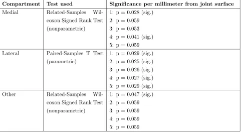
In case of HTO, a nonparametric test showed no significant differences in the MAD in all three compartments. In KJD, not all variables showed a normal distribution in case of MAD so different statistical tests were used. Table 1 shows the results of the parametric and nonparametric tests that were used to determine if KJD had significant change in MAD. Especially in the lateral com-partment significant change in MAD can be found.

Compartment Test used Significance per millimeter from joint surface

Medial Related-Samples Wil-coxon Signed Rank Test (nonparametric)

1: p = 0.028 (sig.) 2: p = 0.059 3: p = 0.053 4: p = 0.041 (sig.) 5: p = 0.059 Lateral Paired-Samples T Test

(parametric)

1: p = 0.029 (sig.) 2: p = 0.025 (sig.) 3: p = 0.026 (sig.) 4: p = 0.027 (sig.) 5: p = 0.029 (sig.) Other Related-Samples

Wil-coxon Signed Rank Test (nonparametric)

[image:12.595.67.549.358.621.2]

1: p = 0.047 (sig.) 2: p = 0.059 3: p = 0.059 4: p = 0.059 5: p = 0.059

(13)

(a) MAD Graph lateral compartment

(b) MAD Graph medial compartment

[image:13.595.154.441.55.646.2]

(c) MAD Graph surface other than lateral and medial compart-ments

Figure 6: Graphs of MAD at baseline and two year follow-up after treatment with HTO or KJD.

(14)

After treatment with HTO, changes in bone density were visible in especially the lateral com-partment. In figure 7 the lateral compartment shows an increase in intensity, and therefore bone density, at the two year follow-up image. After treatment with KJD a change in intensity was also visible. In figure 8 the medial compartment shows a decrease in intensity.

[image:14.595.102.492.148.302.2]

(a) Baseline (b) Two year follow-up

Figure 7: Intensity based colour map of the lateral and medial compartment was reconstructed on tibial plateau. Images of one subject at baseline and two year follow-up after treatment with HTO are shown in HU.

(a) Baseline (b) Two year follow-up

[image:14.595.107.490.381.532.2]

(15)

4 Discussion

The aim of this study is to determine what the influence is of KJD and HTO on the quality of the periarticular bone. This was done by assessment of different variables in different depths of the tibial bone that represent bone density. The mean intensity and the MAD were reviewed for the weight bearing areas underneath the medial and lateral condyles of the femur in particular. The results show that there is no statistical significant difference in mean intensity for all the different areas after both HTO and KJD. However, the results show a slight decrease in intensity after both treatments. The fact that there is no significant change in the mean intensity could be explained by cyst formation in OA. The cysts that are formed in bone tissue have low intensity values on CT images. The bone tissue also contains parts with scleroses that have high values on CT images. Because these values neutralize each other in a mean intensity value, the mean intensity at two year follow-up may not be that much different from the mean intensity calculated at baseline. As a result, change in bone density is harder to statistically prove.

To overcome this effect, this research focusses on the MAD because it displays absolute changes in the bone density. The MAD after KJD significantly decreases in the medial, lateral and other compartments of the tibial plateau. This shows that after the treatment the bone density of the periarticular bone of the tibia neutralizes, meaning the quality shifts towards the quality of healthy bone. This indicates that KJD is a suitable method to treat patients suffering from OA. However, the results of the patients treated with HTO do not show significant changes in the MAD. This can be explained by the fact that HTO is a more invasive procedure which results in more damage to the bone. Because the shift in weight bearing areas caused by HTO, which is the main principle of this procedure, quality improvement of the subchondral and trabecular bone does not necessarily have to occur. As a result of this shift in weight bearing, pressure areas also change. In some scans there was an increase in intensity visible in the lateral compartment due to the increased pressure on this side of the tibial plateau. Since patients treated with HTO have a main affected side, the treatment could help in reducing pain, because HTO showed little decrease in bone density on the main affected side.

4.1 Computed Tomography settings

The displayed HU for a certain structure might not be the same for every scan, since the HU scale is normalized to the brightness and contrast of distilled water at standard pressure and temperature. The Hounsfield scale is linear between two points:

1000×µ(x,y)−µwater

µwater

(1)

(16)

Since the CT images were made before the start of this research, the use of a phantom nor dual energy radiography was possible. For the CT images used in this research the same CT scanner was used and all settings were equal except for the Peak KiloVoltage (kVp) for one patient. The kVp was set at 120 kVp for all patients but one, a value of 100 kVp was chosen for this CT scan. for the scans at baseline and at two year follow-up of that patient that were to be compared with unequal settings, the x-ray spectra were found within a similar window as shown in figure 9. Because of the similar x-ray spectrum it was decided to include these CT scans in the research.

[image:16.595.106.494.213.334.2]

(a) 100 kVp (b) 120 kVp

Figure 9: X-Ray spectrum of the CT-images. In both spectra can be seen that the values focus around the same point, indicating that there is no shift in values due to the difference in kVp.

4.2 Future recommendations

4.2.1 Partial volume effect

An aspect that has to be taken into account when using CT data is the partial volume effect. Because voxels have a certain size, different types of tissue can be captured within the same voxel, resulting in a mean voxel intensity of those tissues. This effect could have had a significant influence on the outcome of this research, since it mainly looked at bone surfaces.

For future research, this effect could be reduced to a minimum by selecting scans with the lowest possible slice thickness.

4.2.2 Ultra thin slices

Just after the script was nearly finished, ultra thin slices were available. These ultra thin slices were made in axial view, instead of the coronal view the script was originally written for. Because ultra thin slices consist of more data, they were expected to be more accurate. Also, the partial volume effect would be reduced when using these ultra thin slices. Therefore, this data was loaded into the script after using the permute function to reconstruct the coronal slices. As a result, the proportions of the images were incorrect and there was more noise after segmentation than in the original coronal slices. To fix these problems, a large part of the script should be rewritten and keeping the time to the deadline in mind, the choice was made to keep using the original, less thin, coronal slices.

(17)

4.2.3 Segmentation

Several threshold methods for segmentation were considered, but eventually a value based on literature study was chosen. This was done because the difference in accuracy for the different methods seemed minimal, the results would be less influenced because the threshold value is the same in every scan and the script was much faster this way. Nevertheless, a more advanced threshold method could improve the segmentation of the bone tissue, especially because the written script is not capable of splitting the bones when the segmented tibia and femur where connected with several voxels. During the research this lead to the exclusion of eight subjects. Since the excluded subjects were of both the KJD and HTO groups, it is assumed that the exclusion did not affect the outcome of this research. For future researches, it is recommended to include a larger population which would increase the validity of the study.

Also, when looking at the results this threshold method seems not fully capable of filtering all soft tissue. The first layer, surface until 1 mm depth, had a very large range of intensity values, which is not expected in bone tissue. When zooming in at the image of this layer, a small layer of one pixel of surrounding soft tissue could be seen. This layer was filtered away with an erode

function in Matlab, but in some cases the segmentation and the erode function created gaps in the tibial bone. Smaller gaps could be closed by using the function imclose in Matlab but this was insufficient for larger gaps. This resulted in a loss of data that could have influenced the outcome of this research. In this research the limited time resulted in imperfect segmented bone.

Since the segmentation of the tibial bone plays such a crucial role in the reconstruction of the tibial plateau, it is essential that this process works as good as possible. For future research the segmented bone should be optimized before continuing the calculations. When the bone contains less gaps and noise the measurements will be more reliable and significant changes will be easier to prove. Perhaps different segmentation methods should be considered apart from threshold-ing. Altogether, a more advanced segmentation method could improve the segmentation step and therefore all following steps in the script.

4.3 Conclusion

(18)

References

[1] Wittenauer R. Smith L. Aden K. Tanna, S. Update on 2004 background paper 6.12 osteoarthritis. http://www.who.int/medicines/areas/priority medicines/BP6 12Osteo.pdf, January 2013. Accessed:

May 9, 2016.

[2] Gommer A. Poos M. Hoe vaak komt artrose voor en hoeveel mensen sterven eraan? http://www. nationaalkompas.nl/gezondheid-en-ziekte/ziekten-en-aandoeningen/bewegingsstelsel-en-bindweefsel/

artrose/omvang/, June 2014. Accessed: April 19, 2016.

[3] James A Martin and Joseph A Buckwalter. Roles of articular cartilage aging and chondrocyte senescence

in the pathogenesis of osteoarthritis. Iowa Orthopaedic Journal, 21:1–7, 2001.

[4] Linda Troeberg and Hideaki Nagase. Proteases involved in cartilage matrix degradation in osteoarth-ritis. Biochimica et Biophysica Acta (BBA)-Proteins and Proteomics, 1824(1):133–145, 2012.

[5] DT Felson, DR Gale, M Elon Gale, J Niu, DJ Hunter, J Goggins, and MP Lavalley. Osteophytes and

progression of knee osteoarthritis. Rheumatology, 44(1):100–104, 2005.

[6] S Milz and Reinhard Putz. Quantitative morphology of the subchondral plate of the tibial plateau.

Journal of anatomy, 185(Pt 1):103, 1994.

[7] Anne Ballinger. Essentials of Kumar and Clark’s Clinical Medicine. Elsevier Health Sciences, 2011.

[8] KM Jordan, NK Arden, Michael Doherty, Bernard Bannwarth, JWJ Bijlsma, Paul Dieppe, K Gunther, Hans Hauselmann, Gabriel Herrero-Beaumont, Phaedon Kaklamanis, et al. Eular recommendations

2003: an evidence based approach to the management of knee osteoarthritis: Report of a task force of

the standing committee for international clinical studies including therapeutic trials (escisit). Annals of the rheumatic diseases, 62(12):1145–1155, 2003.

[9] Dong Chul Lee and Seong Joon Byun. High tibial osteotomy.Knee surgery & related research, 24(2):61– 69, 2012.

[10] Karen Wiegant. Knee joint distraction. intrinsic cartilage repair and sustained clinical benefit. 2015.

[11] JJW Ploegmakers, PM Van Roermund, J Van Melkebeek, Johan Lammens, JWJ Bijlsma, FPJG

Lafeber, and ACA Marijnissen. Prolonged clinical benefit from joint distraction in the treatment of ankle osteoarthritis. Osteoarthritis and cartilage, 13(7):582–588, 2005.

[12] F Intema, TP Thomas, DD Anderson, JM Elkins, TD Brown, A Amendola, FPJG Lafeber, and

CL Saltzman. Subchondral bone remodeling is related to clinical improvement after joint distraction in the treatment of ankle osteoarthritis. Osteoarthritis and Cartilage, 19(6):668–675, 2011.

[13] A Cazenave. High valgus tibial osteotomy. http://www.orthopale.com/tibial-osteotomy.php, 12 2007.

[14] Simon C Mastbergen, Dani¨el BF Saris, and Floris PJG Lafeber. Functional articular cartilage repair:

here, near, or is the best approach not yet clear? Nature reviews rheumatology, 9(5):277–290, 2013.

[15] Joseph J Schreiber, Paul A Anderson, and Wellington K Hsu. Use of computed tomography for assessing

bone mineral density. Neurosurgical focus, 37(1):E4, 2014.

[16] Judith E Adams. Quantitative computed tomography. European journal of radiology, 71(3):415–424, 2009.

[17] F P J G Lafeber and K Wiegant. Trial info: Knee joint distraction in comparison with high tibial

(19)

[18] A. Balter. Dicom23d, in: 3d visualization of density distribution. http://nl.mathworks.com/

matlabcentral/fileexchange/45949-3d-visualization-of-density-distribution?s tid=srchtitle, 2009. Pa-cific Northwest National Laboratory. Accessed: May 10 2016.

[19] Abdal M Alyassin and Gopal B Avinash. Semiautomatic bone removal technique from ct angiography

data. InMedical Imaging 2001, pages 1273–1283. International Society for Optics and Photonics, 2001.

[20] D.J. Kroon. Viewer3d, in: Medical viewer. http://www.mathworks.com/matlabcentral/fileexchange/ 21993-viewer3d, 11 2008.

[21] Alex AT Bui and Ricky K Taira. Medical imaging informatics. Springer Science & Business Media,

(20)

Appendices

Appendix I

Flowchart Methodology

Data of 35 patients were

provided by UMC Utrecht

Data of 32 patients were suited for matlab 3 patients were excluded due

to missing BL or 2 year data

DICOM files were read into matlab

Images were segmented based on thresholding 8 patients were excluded due

to insufficient segmentation

Data of 24 patients were

used to extract results

The femur was extracted from the image matrix

Axial images of tibial plateau were created 1 patient was excluded

because the tibial plateau

was created incorrectly

Measurements and cal-culations were based on

(21)

Appendix II

List of Matlab Commands

Bwconncomp: finds the connecting pixels in 3D space. A value of connectivity can be specified.

Imclose: closes gaps in an image with a specified shape and size.

Imerode: removes specified number of pixels from the boundaries of connected pixels.

Imrect: creates an interactive tool in which the user can select a certain rectangle area using the mouse. Different values can be extracted from the selected area, for example position of the edges and values of the

pixels within the rectangle.

(22)

Appendix III

Matlab Script

1 %% read dicom files

2

3 for g = 1:2

4 clearvars -except g;

5 close all;

6

7 default dicom fields = {...

8 'Filename',...

9 'Height', ... 10 'Width', ...

11 'Rows',...

12 'Columns', ...

13 'PixelSpacing',... 14 'SliceThickness',...

15 'SliceLocation',...

16 'ImagePositionPatient',...

17 'ImageOrientationPatient',...

18 'FrameOfReferenceUID',...

19 };

20

21 % We need these checks because to calculate the "extra fields", we

22 % need to have the PixelSpacing and SliceThickness data. If not, we

23 % leave out the extra fields.

24 no pixel spacing = false; 25 no slice thickness = false;

26

27 extra fields = {...

28 'PhysicalHeight',... % Height (cols) of slice in mm

29 'PhysicalWidth',... % Width (rows) of slice in mm

30 'PixelSliceLocation',... % Slice z-location in pixels

31 'PixelSliceThickness',... % Slice thickness in pixels 32 'SliceData'... % The slice image data

33 };

34 35

36 dicom directory = uigetdir();

37 all fields = [default dicom fields, extra fields];

38

39 % Get directory listing

40 listing = dir(dicom directory);

41 % number of files

42 N = numel(listing); % How many entries in the directory listing 43 if (N<3)

44 error('Empty folder');

45 return

46 end 47

48 slice data(N) = cell2struct(cell(size(all fields)), all fields, 2);

49

(23)

51

52 true index = 0; % a sequential index of dicom files, that is ignoring

53 % files of other types.

54

55 for i = 3:length(listing) % loop through directory listing, but skip '.' and '..'

56 filename = listing(i).name;

57 [dummy path, just the name, extension] = fileparts(filename);

58 full path = fullfile(dicom directory, filename);

59

60 goodfile = false;

61

62 % Check for good dicom file

63 if isdicom(full path)

64 true index = true index + 1;

65 header = dicominfo(full path); 66 slice image = dicomread(header);

67

68 % Save selected header data into the structure slice data

69 for j = 1:numel(default dicom fields) % loop through dicom field names

70 current field = default dicom fields{j};

71 % Deal with requested fields not found in header

72 if isfield(header, current field)

73 slice data(true index).(current field) = header.(current field);

74 else

75 ['header did not contain the field ' current field]

76 end %if

77

78 end % loop through dicom field names

79 % done saving filtered header data

80

81 % Save slice data

82 slice data(true index).SliceData = slice image;

83 % Save extra fields

84 needed header tags = [...

85 isfield(header, 'PixelSpacing'), ...

86 isfield(header, 'SliceThickness'), ...

87 isfield(header, 'SliceLocation')...

88 ];

89

90 if all(needed header tags)

91 pixel spacing = header.PixelSpacing;

92 slice data(true index).PhysicalHeight = ...

93 _{double(pixel spacing(1)*header.Columns);} 94 slice data(true index).PhysicalWidth = ... 95 _{double(pixel spacing(2)*header.Rows);}

96 % need to double check which aspect ratio goes with cols/rows

97 slice data(true index).PixelSliceLocation = ...

98 header.SliceLocation / mean(pixel spacing); 99 slice data(true index).PixelSliceThickness = ...

100 header.SliceThickness / mean(pixel spacing);

101 else

102 no pixel spacing = true;

103 end % if pixel spacing

(24)

105 end % if isdicom

106

107 waitbar(i/N,h);

108 end % loop through directory listing

109 % Eliminate empty structs at end.

110 slice data = slice data(1:true index);

111

112 waitbar(1,h);

113 close(h);

114 warning on;

115

116 % Check that some dicom slice was found

117 if true index < 1

118 'No dicom slices found...returning empty' 119 volume image = [];

120 slice data = [];

121 image meta data = [];

122 return

123 end

124

125 % If SliceLocation is known, sort by that. This is deemed more

126 % accurate than going by filename order (or file number).

127 if isfield(slice data(1), 'SliceLocation')

128 [S,I] = sort([slice data.SliceLocation]);

129 slice data = slice data(I);

130 end 131

132 pixelspacing = round(slice data(true index).PixelSliceThickness);

133 % Pre-allocate volume image array

134 [rows, cols] = size(slice data(1).SliceData);

135 volume image = ...

136 _{zeros(rows, cols, (length(slice data)*pixelspacing));} 137

138 % Build volume image array

139 h = waitbar(0,'Writing slice images to volume image array...','WindowStyle','modal');

140 for i = 1:length(slice data)

141 waitbar(i/N,h);

142 _{volume image(:,:,(i*pixelspacing)) = slice data(i).SliceData;} 143 for j = 1:pixelspacing-1

144 _{volume image(:,:,(i*pixelspacing)-j) = slice data(i).SliceData;} 145 end

146 end

147 close(h);

148 a = size(volume image); 149 num slices = a(3);

150

151 %% Threshold 3d-volume based on value from literature

152 middleslice = round(num slices/2); 153 HU = 306;% Thresholdvalue in HU

154 Threshold = HU + 1024;% Thresholdvalue in grayscale. 1024 is from the dicominfo

155 T = volume image > Threshold;

156 _{VI T1 = volume image .* T;} 157 Threshold2 = Threshold;

(25)

159 se = strel('disk',1);

160 SE = strel('line',3,0);

161 for i = 1:num slices

162 test = VI T1(:,:,i); 163 test = imclose(test,SE);

164 IR = imerode(test,se);

165 VI T(:,:,i) = IR;

166 end

167 %% Filtering & Splitting based on position of labels

168 figure(1), imshow(VI T(:,:,middleslice),[])

169 title('Click inbetween tibia and femur') 170 [xtb, ytb, tbvalue] = impixel

171 close(1)

172

173 Label = bwconncomp(VI T ,18);

174 numlabels = max(size(Label.PixelIdxList));

175 L = zeros([rows,cols,num slices]);

176 n = 1;

177

178 for i = 1:numlabels

179 freq = max(size(Label.PixelIdxList{1,i}));

180 if freq > 10000 181 for j = 1:freq

182 p = Label.PixelIdxList{1,i}(j);

183 L(p) = n;

184 end

185 n = n + 1;

186 end

187 end

188

189 numlabels = max(L(:));

190 FFL = L;

191 for i = 1:numlabels

192 [Y1,X1] = find(L==i); % finding coordinates of areas

193 MY1 = mean(Y1); % mean Y coordinate

194 if MY1 < (ytb)% deleting areas below mean frequency

195 L(L==i) = 0; 196 end

197 end

198 % finding and deleting unwanted stuff

199 figure(1),imshow(L(:,:,middleslice))

200 title('Finding and deleting unwanted stuff, if none: click black')

201 pixel values = impixel;

202 size pixel values = size(pixel values); 203 close(1)

204 if pixel values(1,1) ~= 0

205 for i = 1:size pixel values(1)

206 P = pixel values(i,1);

207 L(L==P) = 0;

208 end

209 end

210 L = logical(L);

(26)

213 %% creating femur location

214 figure(1),imshow(FFL(:,:,middleslice))

215 title('Click femur')

216 pixel values = impixel;

217 pixel values = mean(pixel values);

218 close(1)

219 h = waitbar(0,'Creating femur location','WindowStyle','modal');

220 FL = zeros([10,10]);

222 for j = 1:512

223 for k = 200:512

224 if FFL(513-k,j,i) == pixel values

225 FL(j,i) = 513-k;

226 break

227 else

228 FL(j,i) = 0;

229 end

230 end

231 end

232 waitbar(i/num slices,h)

233 end

234 FL(FL==0) = NaN; 235 close(h);

236 %% finding place where condyles are separted

237 FL1 = uint16(FL);

238 b = bwlabel(FL1); 239 for i = 1:1000

240 flmin = min(FL1(FL1>0));

241 FL1(FL1==flmin) = 0;

242 b = bwlabel(FL1);

243 if max(b(:)) > 1

244 for j = 1:max(b(:))

245 if max(size(find(b==j))) < 100

246 [x,y] = find(b==j);

247 b(b==j) = 0;

248 FL1(x,y) = 0;

249 end

250 end

251 b = bwlabel(b);

252 end

253 if max(b(:)) > 1

254 figure(1),imshow(b,[])

255 bweg = impixel;

256 bweg = mean(bweg); 257 if bweg == 0

258 close(1)

259 cut off = min(FL1(FL1>0));

260 flmin = min(FL1(FL1>0)); 261 FL1(FL1==flmin) = 0;

262 flmin = min(FL1(FL1>0));

263 FL1(FL1==flmin) = 0;

264 break

265 else

(27)

267 for k = 1:max(size(x))

268 FL1(x(k),y(k)) = 0;

269 end

270 end

271 end

272 end

273 condyles = logical(FL1);

274 condyles = imfill(condyles,'holes');

275 %% crop image based on cut off value

276 [X,Y] = find(L==1);

277 cut off = cut off - 15;

278 result cropped = result(cut off:end,:,:);

279 VI cropped = volume image(cut off:end,:,:);

280

281 %% creating tibia plateaus for different layers.

282 info = dicominfo(full path);

283 difY = (512-cut off);

284 difX = 512;

285 num pixels = 10;

286 pixpermm = round((slice data(true index).PixelSliceThickness)/

287 (slice data(true index).SliceThickness));

288 h = waitbar(0,'Creating tibial plateau grayscale-map','WindowStyle','modal'); 289

291 for j = 1:(difX)

292 for k = 1:(difY-(5*pixpermm)) 293 if result cropped(k,j,i) ~= 0

294 for l = 1:pixpermm

295 pixels1(l) = VI cropped((k+(l-1)),j,i);

296 pixels2(l) = VI cropped((k+(l-1)+pixpermm),j,i);

297 _{pixels3(l) = VI cropped((k+(l-1)+(2*pixpermm)),j,i);} 298 _{pixels4(l) = VI cropped((k+(l-1)+(3*pixpermm)),j,i);} 299 pixels5(l) = VI cropped((k+(l-1)+(4*pixpermm)),j,i);

300 end

301 t plat gray(j,i,1) = mean(pixels1);

303 t plat gray(j,i,3) = mean(pixels3); 304 t plat gray(j,i,4) = mean(pixels4);

306 t plat loc(j,i) = k;

307 break

308 else

309 t plat gray(j,i,:) = NaN;

310 t plat loc(j,i) = NaN;

311 end

312 end

313 end

314 waitbar(i/num slices,h) 315 end

316 close(h)

317 H1=t plat gray(:,:,1);H2=t plat gray(:,:,2);H3=t plat gray(:,:,3);H4=t plat gray(:,:,4);

318 H5=t plat gray(:,:,5);

319 montage1 = [H1 H2 H3 H4 H5];

(28)

321 %% deleting holes from tibia plateau location

322 TPL = 512 - t plat loc;

323

324 depth = 10;

325 _{cut off1 = mode(TPL(:))-(depth*pixpermm);} 326 TPL(TPL<cut off1) = 0;

327 imshow(TPL,[])

328 %creating logical of tibia plateau

329 TPL(isnan(TPL))=0;

330 TPlogical = bwlabel(TPL,8);

331 num labels = max(TPlogical(:)); 332 for i = 1:num labels

333 freq(i) = max(size(find(TPlogical(TPlogical==i))));

334 end

335 maxfreq = find(freq==max(freq(:))); 336 TPlogical(TPlogical~=maxfreq) = 0; 337 TPlogical = logical(TPlogical);

338 %creating logical of condyles(lateral and medial)

339 TPG = t plat gray(:,:,1);

340 num layers = 5;

341 b = bwlabel(condyles);

342 figure(1) 343 imshow(TPG,[])

344 figure(2)

345 imshow(b)

346 title('Select lateral condyle') 347 pixlatcon = impixel;

348 close([1 2])

349 pixlatcon = pixlatcon(1,1);

350 bm = b;

351 bm(bm==pixlatcon) = 0;

352 bm = logical(bm);

353 bl = b;

354 bl(bl~=pixlatcon) = 0; 355 bl = logical(bl);

356 rest = ~condyles;

357 rest = logical(rest); 358 %%

359 for i = 1:5

360 TPG = t plat gray(:,:,i);

361 _{TPG = TPG.*TPlogical;} 362 plateaus(:,:,i) = TPG;

363 end

364

365 %% Save data

366 fileloc = char(dicom directory);

367 filename = [ fileloc '.mat' ];

368 save(filename,'num slices',... 369 'volume image',...

370 'info',...

371 'result cropped',...

372 'TPL',...

373 'condyles',...

(29)

375 'bm',...

376 'bl',...

377 'rest'...

378 ); 379

380 end

1 % open saved data

2 clear all

3

4 voor = load(['VOOR.mat']);

5 na = load(['NA.mat']);

6 %% selecting which condyles you want to use

7 montage = [voor.condyles na.condyles];

8 figure(1)

9 imshow(montage,[])

10 title('Voor Na')

11 prompt = 'Which condyles do you want to use?? ';

12 str = input(prompt,'s');

13 close(1)

14

15 if strcmp(str,'voor') == 1

16 welke is wat = 'voor is fixed'; 17 condyles = voor.condyles;

18 bm = voor.bm;

19 bl = voor.bl;

20 rest = voor.rest; 21 Fixed = voor.plateaus;

22 Moving = na.plateaus;

23 else

24 welke is wat = 'na is fixed';

25 condyles = na.condyles;

26 bm = na.bm;

27 bl = na.bl; 28 rest = na.rest;

29 Fixed = na.plateaus;

30 Moving = voor.plateaus;

31 end

32 %% imregister before and after

33 for k = 1:5

34 fixed = uint16(Fixed(:,:,k));

35 moving = uint16(Moving(:,:,k));

36

37 [optimizer, metric] = imregconfig('monomodal');

38 MR(:,:,k) = imregister(moving,fixed,'affine',optimizer,metric); 39 end

40 %% calculating different values for fixed

41 for i = 1:5

42 TPG = Fixed(:,:,i); 43

44 A = TPG;

(30)

47 _{Rest = A.*rest;} 48 _{TPGC = A.*condyles;} 49

50 meantotal = round(mean(A(A>0))); 51 modustotal = mode(A(A>0));

52 MADtotal = round(nanmean(mad(A)));

53 skewtotal = skewness(A(:));

54 kurttotal = kurtosis(A(:));

55

56 meanmedial = round(mean(TPGM(TPGM>0)));

57 modusmedial = mode(TPGM(TPGM>0)); 58 MADmedial = round(nanmean(mad(TPGM)));

59 skewmedial = skewness(TPGM(:));

60 kurtmedial = kurtosis(TPGM(:));

61

62 meanlateral = round(mean(TPGL(TPGL>0)));

63 moduslateral = mode(TPGL(TPGL>0));

64 MADlateral = round(nanmean(mad(TPGL)));

65 skewlateral = skewness(TPGL(:));

66 kurtlateral = kurtosis(TPGL(:));

67

68 meanrest = round(mean(Rest(Rest>0))); 69 modusrest = mode(Rest(Rest>0));

70 MADrest = round(nanmean(mad(Rest)));

71 skewrest = skewness(Rest(:));

72 kurtrest = kurtosis(Rest(:)); 73

74 meancondyles = round(mean(TPGC(TPGC>0)));

75 moduscondyles = mode(TPGC(TPGC>0));

76 MADcondyles = round(nanmean(mad(TPGC)));

77 skewcondyles = skewness(TPGC(:));

78 kurtcondyles = kurtosis(TPGC(:));

79

80 mean values fixed(i) = struct('meantotal',meantotal,'modustotal',modustotal,'MADtotal',MADtotal,

81 'skewtotal',skewtotal,'kurttotal',kurttotal,...

82 'meanmedial',meanmedial,'modusmedial',modusmedial,'MADmedial',MADmedial,'skewmedial',

83 skewmedial,'kurtmedial',kurtmedial,...

84 'meanlateral',meanlateral,'moduslateral',moduslateral,'MADlateral',MADlateral,'skewlateral',

85 skewlateral,'kurtlateral',kurtlateral,...

86 'meancondyles',meancondyles,'moduscondyles',moduscondyles,'MADcondyles',MADcondyles,

87 'skewcondyles',skewcondyles,'kurtcondyles',kurtcondyles,...

88 'meanrest',meanrest,'modusrest',modusrest,'MADrest',MADrest,'skewrest',skewrest,'kurtrest',

89 kurtrest);

90 end

91 %% calculating different values for movingregistered

92 MR = double(MR);

93 for i = 1:5

94 TPG = MR(:,:,i); 95

96 A = TPG;

(31)

101

102 meantotal = round(mean(A(A>0)));

103 modustotal = mode(A(A>0));

104 MADtotal = round(nanmean(mad(A))); 105 skewtotal = skewness(A(:));

106 kurttotal = kurtosis(A(:));

107

108 meanmedial = round(mean(TPGM(TPGM>0)));

109 modusmedial = mode(TPGM(TPGM>0));

110 MADmedial = round(nanmean(mad(TPGM)));

111 skewmedial = skewness(TPGM(:)); 112 kurtmedial = kurtosis(TPGM(:));

113

114 meanlateral = round(mean(TPGL(TPGL>0)));

115 moduslateral = mode(TPGL(TPGL>0)); 116 MADlateral = round(nanmean(mad(TPGL)));

117 skewlateral = skewness(TPGL(:));

118 kurtlateral = kurtosis(TPGL(:));

119

120 meanrest = round(mean(Rest(Rest>0)));

121 modusrest = mode(Rest(Rest>0));

122 MADrest = round(nanmean(mad(Rest))); 123 skewrest = skewness(Rest(:));

124 kurtrest = kurtosis(Rest(:));

125

126 meancondyles = round(mean(TPGC(TPGC>0))); 127 moduscondyles = mode(TPGC(TPGC>0));

128 MADcondyles = round(nanmean(mad(TPGC)));

129 skewcondyles = skewness(TPGC(:));

130 kurtcondyles = kurtosis(TPGC(:));

131 %save calculated data to struct

132 mean values MR(i) = struct('meantotal',meantotal,'modustotal',modustotal,'MADtotal',MADtotal,

133 'skewtotal',skewtotal,'kurttotal',kurttotal,...

134 'meanmedial',meanmedial,'modusmedial',modusmedial,'MADmedial',MADmedial,'skewmedial',

135 skewmedial,'kurtmedial',kurtmedial,...

136 'meanlateral',meanlateral,'moduslateral',moduslateral,'MADlateral',MADlateral,'skewlateral',

137 skewlateral,'kurtlateral',kurtlateral,...

138 'meancondyles',meancondyles,'moduscondyles',moduscondyles,'MADcondyles',MADcondyles,

139 'skewcondyles',skewcondyles,'kurtcondyles',kurtcondyles,...

140 'meanrest',meanrest,'modusrest',modusrest,'MADrest',MADrest,'skewrest',skewrest,'kurtrest',

141 kurtrest);

142 end

143 %% renaming fixed and MR

144 if strcmp(str,'voor') == 1 145 MVvoor = mean values fixed;

146 MVna = mean values MR;

147 else

148 MVvoor = mean values MR; 149 MVna = mean values fixed;

150 end

151 %%

152 MR = double(MR);

153 for i = 1:5

(32)

155 for k = 1:size(Fixed,2)

156 if Fixed(j,k,i) == 0

157 diff(j,k,i) = 0;

158 elseif MR(j,k,i) == 0

159 diff(j,k,i) = 0;

160 else

161 if strcmp(str,'voor') == 1

162 diff(j,k,i) = abs(Fixed(j,k,i) - MR(j,k,i));

163 else

164 diff(j,k,i) = abs(MR(j,k,i) - Fixed(j,k,i));

165 end

166 end

167 end

168 end

169 end 170 %%

171 diff(isnan(diff)) = 0;

172 se = strel('disk',1);

173 for i = 1:5

174 test = diff(:,:,i);

175 IR = imerode(test,se);

176 diff(:,:,i) = IR;

Change in 3d periarticular bone density after Knee Joint Distraction or High Tibial Osteotomy in the treatment of osteoarthritis

Bachelor Thesis Technical Medicine

Multidisciplinary Assignment