Original citation:
Hart, Sergiu, Kremer, Ilan and Perry, Motty (2015) Evidence games : truth and commitment. Working Paper. Coventry: Department of Economics, University of Warwick. Warwick Economics Research Paper Series (WERPS) (1091). (Unpublished)
Permanent WRAP URL:
http://wrap.warwick.ac.uk/82306
Copyright and reuse:
The Warwick Research Archive Portal (WRAP) makes this work by researchers of the University of Warwick available open access under the following conditions. Copyright © and all moral rights to the version of the paper presented here belong to the individual author(s) and/or other copyright owners. To the extent reasonable and practicable the material made available in WRAP has been checked for eligibility before being made available.
Copies of full items can be used for personal research or study, educational, or not-for-profit purposes without prior permission or charge. Provided that the authors, title and full bibliographic details are credited, a hyperlink and/or URL is given for the original metadata page and the content is not changed in any way.
A note on versions:
The version presented here is a working paper or pre-print that may be later published elsewhere. If a published version is known of, the above WRAP url will contain details on finding it.
Warwick Economics Research Paper Series
Evidence Games: Truth and
Commitment
Sergiu Hart, Ilan Kremer & Motty Perry
December, 2015
Evidence Games: Truth and Commitment
1
Sergiu Hart
2Ilan Kremer
3Motty Perry
4July 12, 2015
1First version: February 2014. The authors thank Elchanan Ben-Porath, Peter
DeMarzo, Kobi Glazer, Johannes H¨orner, Vijay Krishna, Phil Reny, Ariel Rubin-stein, Amnon Schreiber, Andy Skrzypacz, Rani Spiegler, Yoram Weiss, and David Wettstein, for useful comments and discussions.
2Department of Economics, Institute of Mathematics, and Federmann
Cen-ter for the Study of Rationality, The Hebrew University of Jerusalem. Re-search partially supported by an Advanced Investigator Grant of the Eu-ropean Research Council (ERC). E-mail: [email protected] Web site:
http://www.ma.huji.ac.il/hart
3Department of Economics, Business School, and Federmann Center for the
Study of Rationality, The Hebrew University of Jerusalem; Department of Eco-nomics, University of Warwick. Research partially supported by a Grant of the European Research Council (ERC). E-mail: [email protected]
4Federmann Center for the Study of Rationality, The
He-brew University of Jerusalem; Department of Economics, Univer-sity of Warwick. E-mail: [email protected] Web site:
Abstract
1
Introduction
Ask someone if they deserve a pay raise. The invariable reply (with very few, and therefore notable, exceptions) is, “Of course I do.” Ask defendants in court whether they are guilty and deserve a harsh punishment, and the again invariable reply is, “Of course not.”
So how can reliable information be obtained? How can those who de-serve a reward, or a punishment, be distinguished from those who do not? Moreover, how does one determine the right reward or punishment when ev-eryone, regardless of information and type, prefers higher rewards and lower punishments?1
These are clearly fundamental questions, pertinent to many important setups. The original focus in the relevant literature was on equilibrium and equilibrium prices. This approach was initiated by Akerlof (1970), and fol-lowed by the large body of work on voluntary disclosure, starting with Gross-man and Hart (1980), GrossGross-man (1981), Milgrom (1981), and Dye (1985). In a different line, the same problem was considered by Green and Laffont (1986) from a general mechanism-design viewpoint, in which one can commit in advance to a policy.
As is well known, commitment is a powerful device.2 The present
pa-per nevertheless identifies a natural and important class of setups—which includes voluntary disclosure as well as various other models of interest— that we call “evidence games,” in which the possibility to commit does not
matter, namely, the equilibrium and the optimal mechanism coincide. This issue of whether commitment can help was initially addressed by Glazer and Rubinstein (2004, 2006).3
Anevidence game is a standard communication game between an “agent” who is informed and sends a message (that does not affect the payoffs) and
1Thus “single-crossing”-type properties do not hold here, which implies that usual separation methods (as in signaling, etc.; see Section 1.2) cannot help.
2Think for instance of the advantage that it confers in bargaining, and in oligopolistic competition (Stackelberg vs. Cournot). See also Example 3 in Section 1.1 that is closer to our setup.
a “principal” who chooses the action (call it the “reward”). The two dis-tinguishing features of evidence games are, first, that the agent’s private information (the “type”) consists of certain pieces of verifiable evidence, and the agent can reveal in his message all this evidence (the “whole truth”), or only some part of it (a “partial truth”).4 The second feature is that the
agent’s preference order on the rewards is the same regardless of his type—he always prefers the reward to be as high as possible5—whereas the principal’s
utility, which does depend on the type, is single-peaked with respect to the agent’s order—he prefers the reward to be as close as possible to the “right reward.” Voluntary disclosure games, in which the right reward is the con-ditional expected value, obtain when the principal (who may well stand for the “market”) has quadratic-loss payoff functions (we refer to this as the “basic case”). See the end of the Introduction for more on this and further applications.
The possibility of revealing the whole truth, an essential feature of evi-dence games, allows one to take into account the natural property that the whole truth has a slight inherent advantage. This is expressed by infinitesi-mal increases6in the agent’s utility and in the probability of telling the whole
truth. Specifically, (i) when the reward for revealing some partial truth is the same as the reward for revealing the whole truth, the agent prefers to reveal the whole truth; and (ii) there is a small positive probability that the whole truth is revealed.7 These conditions, which are part of the setup, and are calledtruth-leaning, are most natural. The truth is after all a focal point, and there must be good reasons for not telling it.8 As Mark Twain wrote,
“When in doubt, tell the truth,” and “If you tell the truth you don’t have to remember anything.”9 With truth-leaning, the resulting equilibria turn out
4
Try to recall the number of job applicants who included rejection letters in their files. 5This is why adding (cheap-talk) messages that any type can use does not help here: all types will use those messages that yield the highest rewards.
6Formally, by limits as these increases go to zero.
7For example, the agent may be nonstrategic with small but positive probability; cf. Kreps, Milgrom, Roberts, and Wilson (1982).
8Psychologists refer to the “sense of well-being” associated with telling the truth. 9
to be precisely those used in the voluntary disclosure literature; moreover, they satisfy the various refinement conditions offered in the literature.10 See
the examples and the discussion in Section 1.1.
The interaction between the two players may be carried out in two distinct ways. One way is for the principal to decide on the reward onlyafterreceiving the agent’s message; the other way is for the principal tocommit to a reward policy, which is made known before the agent sends his message.11,12 The
resulting equilibria will be referred to asequilibria without commitment, and
optimal mechanisms with commitment, respectively. We can now state the main equivalence result.
In evidence games the equilibrium outcome obtained without com-mitment coincides with the optimal mechanism outcome obtained with commitment.
Section 1.1 below provides two simple examples that illustrate the result and the intuition behind it.
An important consequence of the equivalence is that, in the basic case (where the reward equals the conditional expected value), the equilibria yield
constrained Pareto efficient outcomes (i.e., outcomes that are Pareto efficient under the incentive constraints).13 In general, the fact that commitment is
not needed in order to obtain optimality is a striking feature of evidence games. Moreover, we will show that the “truth structure” of evidence games (which consists of the partial truth relation and truth-leaning) is indispens-able for this result.
We stated above that evidence games constitute a very naturally oc-curring environment, which includes a wide range of applications and well-studied setups of much interest. We discuss three such applications. The
10Such as the “intuitive criterion” of Cho and Kreps (1987), “divinity” and “universal divinity” of Banks and Sobel (1987), and the “never weak best response” of Kolberg and Mertens (1986).
11The latter is a
Stackelbergsetup, with the principal as leader and the agent as follower. 12Interestingly, what distinguishes between “signaling” and “screening” (see Section 1.2 below) is precisely these two different timelines of interaction.
first one deals with voluntary disclosure in financial markets. Public firms enjoy a great deal of flexibility when disclosing information. While disclos-ing false information is a criminal act, withholddisclos-ing information is allowed in some cases, and is practically impossible to detect in other cases. This has led to a growing literature in financial economics and accounting (see for example Dye 1985 and Shin 2003, 2006) on voluntary disclosure and its impact on asset pricing. What our result says is that the market’s behavior in equilibrium is in fact optimal: it yields the optimal separation that may be obtained between “good” and “bad” firms (i.e., even if mechanisms and commitments were possible they could not be separated more).
The second application has to do with the legal doctrine known as “the right to remain silent.” In the United States, this right was enshrined in the Fifth Amendment to the Constitution, and is interpreted to include the provision that adverse inferences cannot be made, by the judge or the jury, from the refusal of a defendant to provide information. While the right to remain silent is now recognized in many of the world’s legal systems, its above interpretation regarding adverse inference has been questioned and is not universal. The present paper sheds light on this debate. Indeed, because equilibria entail (Bayesian) inferences, our result implies that the same infer-ences apply to the optimal mechanism. Therefore adverse inferinfer-ences should be allowed, and surely not committedly disallowed. In England, an additional provision (in the Criminal Justice and Public Order Act of 1994) states that “it may harm your defence if you do not mention when questioned something which you later rely on in court,” which may be viewed, on the one hand, as allowing adverse inference, and, on the other hand, as making the revelation of only partial truth possibly disadvantageous—which is the same as giving an advantage to revealing the whole truth (i.e., truth-leaning).
The third application concerns medical overtreatment, which is one of the more serious problems in many health systems in the developed world; see Brownlee (2008).14 A reason that doctors and hospitals overtreat may be
fear of malpractice suits; but the more powerful reason is that they are paid
more for doing so. One suggestion for overcoming this is to reward doctors for providing evidence. The present paper takes a small step towards a better understanding of an optimal incentive scheme designed to reward revelation of evidence in these and other applications.
To summarize the main contribution of the present paper: first, the class of evidence games that we consider models very common and important se-tups in information economics, sese-tups that lie outside the standard signaling and cheap talk literature; second, we prove the equivalence between equi-librium without commitment and optimal mechanism with commitment in evidence games (which, in the basic case of quadratic loss, implies that the equilibria are constrained Pareto efficient); and third, we show that the con-ditions of evidence games—most importantly, the truth structure—are the
indispensable conditions beyond which this equivalence no longer holds. The paper is organized as follows. After the Introduction (which continues below with some examples and a survey of relevant literature), we describe the model and the assumptions in Section 2. The main equivalence result is then stated in Section 3, and proved in Section 4. We conclude with dis-cussions on various extensions and connections in Section 5. The Appendix shows that our conditions are indispensable for the result (Section A.1), and provides a useful alternative proof of one direction of the equivalence result (Section A.2).
1.1
Examples
We provide here two simple examples that illustrate the equivalence result and explain some of the intuition behind it.
Example 1 (A simple version of the model introduced by Dye 1985.) A professor negotiates his salary with the dean. The dean would like to set the salary as close as possible to the professor’s expected market value,15
15Formally, the dean wants to minimize (x
−v)2, where x is the salary and v is the professor’s value; the dean’s optimal response to any evidence is thus to choose x to be the conditional expected value of the types that provide this evidence.
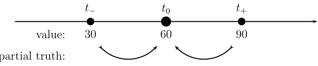
while the professor would naturally like his salary to be as high as possible. The dean, knowing that similar professors’ salaries range between, say, 0 and 120, asks the professor if he can provide some evidence of his “value” (such as whether a recent paper was accepted or rejected, outside offers, and so on). Assume that with probability 50% the professor has no such evidence, in which case his expected value is 60, and with probability 50% he does have some evidence. In the latter case it is equally likely that the evidence is positive or negative, which translates into an expected value of 90 and 30,
respectively. Thus there are three professor types: the “no-evidence” type
t0, with probability 50% and value 60, the “positive-evidence” typet+, with
probability 25% and value 90, and the “negative-evidence” type t−, with probability 25% and value 30. See Figure 1.
30 60 90
t− t0 t+
value:
[image:10.595.112.434.375.442.2]partial truth:
Figure 1: Values and possible partial truth messages in Example 1
Consider first the game setup (without commitment): the professor de-cides whether to reveal his evidence, if he has any, and then the dean chooses the salary.It is easy to verify that there is a unique sequential equilibrium,16
where a professor with positive evidence reveals it and is given a salary of 90 (equal to his value), whereas one with negative evidence conceals it and pretends that he has no evidence. When no evidence is presented the dean’s optimal response is to set the salary at 50, which is the expected value of the
The same applies when the dean is replaced by the “market.” 16
Indeed, in a sequential equilibrium the salary of a professor providing positive evidence must be 90 (because the positive-evidence type is the only one who can provide such evidence), and similarly the salary of someone providing negative evidence must be 30.
two types that provide no evidence: the no-evidence type together with the negative-evidence type.17 See Figure 2.
30 60 90
t− t0 t+
value:
partial truth:
prof. says:
[image:11.595.115.435.199.323.2]dean pays: 30 50 90
Figure 2: Equilibrium in Example 1
Next, consider the mechanism setup (with commitment): the dean com-mits to a salary policy (specifically: three salaries, denotedx+, x−,andx0,for
those who provide, respectively, positive evidence, negative evidence, and no evidence), and then the professor decides what evidence to reveal. One possi-bility is of course the above equilibrium, namely,x+ = 90 andx−=x0 = 50.
Can the dean do better by committing? Can he provide incentives to the negative-evidence type to reveal his information? In order to separate be-tween the negative-evidence type and the no-evidence type, he must give them distinct salaries, i.e., x− 6=x0. But then the salary for those who
pro-vide negative epro-vidence must be higher than the salary for those who propro-vide no evidence (i.e., x− > x0), because otherwise (i.e., when x− < x0) the
negative-evidence type will pretend that he has no evidence and we are back to the no-separation case. Since the value 30 of the negative-evidence type is lower than the value 60 of the no-evidence type, setting a higher salary for the former than for the latter cannot be optimal (indeed, increasing x− and/or decreasing x0 is always better for the dean, as it sets the salary of at least
one type closer to its value). The conclusion is that an optimal mechanism
cannot separate the negative-evidence type from the no-evidence type,18 and
17
The conditional expectation is (50%·60 + 25%·30)/(50% + 25%) = 50.
18
so the unique optimal policy is identical to the equilibrium outcome, which is obtained without commitment. ¤
The following slight variant of Example 1 shows the use of truth-leaning; the requirement of being a sequential equilibrium no longer suffices here.
Example 2 Replace the positive-evidence type of Example 1 by two types: a (new) positive-evidence type t+ with value 102 and probability 20%, and
a “medium-evidence” type t± with value 42 and probability19 5%. The type
t± has two pieces of evidence: one is the same positive evidence that t+
has, and the other is the same negative evidence that t− has (for example, an acceptance decision on one paper, and a rejection decision on another). Thus,t± may pretend to be any one of the four typest±, t+, t−,ort0.In the
sequential equilibrium that is similar to that of Example 1, types t+ and t±
both provide positive evidence and get the salaryx+ = 90 (their conditional
expectation), and types t0 and t− provide no evidence, and get the salary
x0 = 50 (their conditional expectation). It is not difficult to see that this is
also the optimal mechanism outcome.
Now, however, the “babbling equilibrium” (in which the professor, re-gardless of his type, never provides any evidence, and the dean ignores any evidence that might be provided and sets the salary at the average value of 60—clearly, this is worse for the dean as it yields no separation between the types) is a sequential equilibrium. This is supported by the dean’s belief that it is much more probable that the out-of-equilibrium positive evidence is provided by t± rather than by t+; such a belief, while possible in a
se-quential equilibrium, appears hard to justify.20 The babbling equilibrium is
not, however, a truth-leaning equilibrium, as truth-leaning implies that the
the former has a higher value. In general, separation of types with more evidence from types with less evidence can occur in an optimal mechanism only when the former have higher values than the latter (since someone with more evidence can pretend to have less evidence, but not the other way around). In short,separation requires that more evidence be associated with higher value. See Corollary 3 for a formal statement of this property, which is at the heart of our argument.
19There is nothing special about the specific numbers that we use.
out-of-equilibrium messaget+is used infinitesimally by type t+ (for which it
is the whole truth), and so the reward there must be set at 102, the value of21 t
+. ¤
Communication games, which include evidence games, are notorious for their multiplicity of equilibria. Requiring the equilibria to be sequential may eliminate some of them, but in general this is not enough (cf. Shin 2003). Truth-leaning, which we view as part of the “truth structure” that is char-acteristic of evidence games, thus provides a natural equilibrium refinement criterion. See Section 2.3.1.
Finally, lest some readers think that commitment is not useful in the general setup of communication games, we provide a simple variant of our examples—one that does not belong to the class of evidence games—where commitment yields outcomes that are strictly better than anything that can be achieved without it.
Example 3 There are only two types of professor, and they are equally-likely: t0,with no evidence and value 60, andt−,with negative evidence and
value 30. As above, the dean wants to set the salary as close as possible to the value, and t0 wants as high a salary as possible. However, t− now wants
his salary to be as close as possible to 50 (for instance, getting too high a salary would entail duties that he does not like).22
There can be no separation between the two types in equilibrium, since that would imply that t0 gets a salary of 60 and t− gets a salary of 30—but
then t− would prefer not to reveal his evidence and get 60 too. Thus the babbling equilibrium where no evidence is provided and the salary is set at 45, the average of the two values, is the unique Nash equilibrium.
21While taking the posterior belief at unused messages to be the conditional prior would suffice to eliminate the babbling equilibrium here (because the belief at messaget+ would be 80%−20% ont+ andt±), this would not suffice in general; see Example 8 in Section A.1.4.
22Formally, the utility oft− when he gets salaryxis
Consider now the mechanism where the salary policy is to pay 30 when negative evidence is provided, and 75 when no evidence is provided. Since
t−prefers 30 to 75, he will reveal his evidence, and so separation is obtained. The mechanism outcome is better for the dean than the equilibrium outcome (he makes an error of 15 for t0 only in the mechanism, and an error of 15 for
both types in equilibrium).23 The mechanism requires the dean to commit to
pay 75 when he gets no evidence; otherwise, after getting no evidence (which happens when the type is t0),he will want to change his decision and pay 60
instead. ¤
To put it formally, commitment is required when implementing reward schemes that arenot ex-post optimal. Our paper will show that this does not happen in evidence games (the requirement that is not satisfied in Example 3 is that the agent’s utility be the same for all types—see Section A.1.5 in the Appendix; Section A.1.6 there provides another example where commitment yields strictly better outcomes).
1.2
Related Literature
There is an extensive and insightful literature addressing the interaction be-tween a principal who takes a decision but is uninformed and an agent who is informed and communicates information, either explicitly (through mes-sages) or implicitly (through actions). Separation between different types of the agent may indeed be obtained when they have different utilities and costs: signaling (Spence 1973 in economics and Zahavi 1975 in biology), screening (Rothschild and Stiglitz 1976), cheap talk (Crawford and Sobel 1982, Krishna and Morgan 2007).24
When the agent’s utility does not however depend on his information, in order to get any separation the agent’s utility would need to depend on
23The
optimal mechanism pays a salary of 70 for no evidence.
his communication. A simple and standard way of doing this is for different types to have different sets of possible messages.25
First, in the game setup where the agent moves first, Grossman and O. Hart (1980), Grossman (1981), and Milgrom (1981) initiated the voluntary disclosure literature. These papers consider a salesperson who has private information about a product, which he may, if he so chooses, report to a potential buyer. The report is verifiable, that is, the salesperson cannot misreport the information that he reveals; he can however conceal it and not report it. These papers show that in every sequential equilibrium the salesperson employs a strategy of full disclosure: this is referred to as “un-raveling.” The key assumption here that yields this unraveling is that it is commonly known that the agent is fully informed. This assumption was later relaxed, as described below.
Disclosure in financial markets by public firms is a prime example of vol-untary disclosure. This has led to a growing literature in accounting and finance. Dye (1985) and Jung and Kwon (1988) study disclosure of account-ing data. These are the first papers where it is no longer assumed that the agent (in this case, the firm, or, more precisely, the firm’s manager) is known to be fully informed. They consider the case where the information is one-dimensional, and show that the equilibrium is based on a threshold: only types who are informed and whose information is above a certain threshold disclose their information. Shin (2003, 2006), Guttman, Kremer, and Skry-pacsz (2014), and Pae (2005) consider an evidence structure in which infor-mation is multi-dimensional.26 Since such models typically possess multiple
equilibria, these papers focus on what they view as the more natural equilib-rium. The selection criteria that they employ are model-specific. However, it may be easily verified that all these selected equilibria are in fact “truth-leaning” equilibria; thus truth-leaning turns out to be a natural way to unify all these criteria.
25
Which is the same as taking the cost of the message to be zero when it is feasible, and infinite when it isn’t.
26
Second, in the mechanism-design setup where the principal commits to a reward policy before the agent’s message is sent, Green and Laffont (1986) were the first to consider the setup where types differ in the sets of possible messages that they can send. They show that a necessary and sufficient condition for the revelation principle to hold for any utility functions27is that
the message structure be transitive and reflexive—which is satisfied by the voluntary disclosure models, as well as by our more general evidence games. Ben-Porath and Lipman (2012) characterize the social choice functions that can be implemented when agents can also supply hard proofs about their types.
The approach we are taking of comparing equilibria with optimal mech-anisms originated in Glazer and Rubinstein (2004, 2006). They analyze the optimal mechanism-design problem for general type-dependent message structures, with the principal taking a binary decision of “accepting” or “re-jecting”; the agent, regardless of his type, prefers acceptance to rejection. In their work they show that the resulting optimal mechanism can be supported as an equilibrium outcome. More recently, Sher (2011) has provided condi-tions (namely, concavity) under which the result holds when the principal’s decision is no longer binary. See Section 5.3 for a detailed discussion of the Glazer–Rubinstein setup.
Our paper shows that, in the framework of agents with identical utili-ties, the addition of the natural truth structure of evidence games—i.e., the partial truth relation and the inherent advantage of the whole truth—yields a stronger result, namely, the equivalence between equilibria and optimal mechanisms.
2
The Model
The model is a communication game in which the set of messages is the set of types and the set of actions is the real line R. The voluntary disclosure models (Grossman 1981, Milgrom 1981, Dye 1985, 1988, Shin 2003, 2006)
are all special cases of this model.
There are two players, an agent (“A”) and a principal (“P”). The agent’s information is his type t, which belongs to a finite set T, and is chosen according to a given distribution p∈ ∆(T) with full support.28 The
principal knows the distributionpbut does not know the realized type (which the agent does know).
The general structure of the interaction is that the agent sends amessage, which consists of a type s in T, and the principal chooses an action, which consists of a real number x in R. The message is costless: it does not affect the payoffs of the agent and the principal. The next sections will provide the details, including in particular the timeline of the interaction.
The interpretation to keep in mind is that the type is the (verifiable) evidence that the agent possesses, and the message is the evidence that he reveals.
2.1
Payoffs and Single-Peakedness
A basic assumption of the model (which distinguishes it from the signaling and cheap-talk setups) is that all the types of the agent have the same pref-erence, which is strictly increasing in x (and does not, as already stated, depend on the message sent). Since only the ordinal preference of the agent matters,29 we assume without loss of generality that the agent’s payoff is x
itself,30 and refer to x also as the reward (to the agent).
As for the principal, his utility does depend on the typet,but, again, not on the messages; thus, letht(x) be the principal’s utility31for typet ∈T and
reward x ∈ R (and any message s ∈ T). For every probability distribution
q = (qt)t∈T ∈ ∆(T) on the set of types T—think of q as a “belief” on the
28∆(T) :=
{p= (pt)t∈T ∈RT+ :
P
t∈Tpt= 1} is the set of probability distributions on
the finite set T.Full support means thatpt>0 for everyt∈T.
29
See Section 5.2 for randomized rewards. 30
Formally, let the agent’s utility beUA(x, s;t),wherex
∈Ris the action,s∈T is the message, and t∈T is the type. ThenUA(x, s;t) is, for everyt
∈T, a strictly increasing functiongt(x) ofx; without loss of generality,gt(x) =xfor alltandx.
31Formally, writing UP(x, s;t) for the principal’s utility when the action isx
∈R,the message is s∈T,and the type is t∈T,we have UP(x, s;t) =h
space of types—the expected utility of the principal is given, for every reward
x∈R, by
hq(x) :=
X
t∈T
qtht(x).
The functionshtare assumed to bedifferentiable (in the relevant domain,
which will turn out to be a compact interval; see Remark (a) below), and to satisfy a single-peakedness condition. A differentiable real function f : R→R is single-peaked if there exists a point v ∈ R such that f′
(v) = 0;
f′
(x)>0 forx < v; and f′
(x)<0 for x > v. Thusf has a single peak atv,
and it strictly increases when x < v and strictly decreases when x > v. The assumption on the principal’s payoffs is:
(SP) Single-Peakedness. The expected utility of the principal hq(x) is a
single-peaked function of the rewardxfor every probability distribution
q ∈∆(T) on the set of types T.
Thus, (SP) requires each function ht to be single-peaked, and also each
weighted average of such functions to be single-peaked. Let v(t) and v(q) denote the single peaks of ht and hq. Thus,v(t) is the reward that the
prin-cipal views as most fitting, or “ideal,” for type32t; similarly,v(q) is the ideal
reward when the types are distributed according to q.When the distribution of types is given by the prior p, we will at times write v(T) instead of v(p),
and, more generally, v(S) instead of v(p|S) for S ⊆ T (where p|S ∈ ∆(T) denotes the conditional of pgiven33 S).
Basic Example: Quadratic Loss. A particular case, common in much of the literature, uses for each type the quadratic distance from the ideal point: ht(x) =−(x−v(t))2 for eacht ∈T.In this case, for each distribution
q ∈∆(T),the functionhq has its single peak at the expectation with respect
to q of the peaks v(t); i.e., v(q) =Pt∈T qtv(t).
More generally, for each type t ∈ T let ht be a strictly concave function
32We will at times refer tov(t) also as the
value of typet(recall the examples in Section 1.1 in the Introduction).
33(p
|S)t = pt/p(S) for t ∈ S and (p|S)t = 0 for t /∈ S, where p(S) = Pt∈Spt is the
that attains its (unique) maximum at a finite point,34denoted by v(t). Since
any weighted average of such functions clearly satisfies the same properties, the single-peakedness condition (SP) holds.35 For instance, take h
tto be the
negative of some distance from the ideal point v(t). Even more broadly, the (SP) condition allows one to treat types differently, such as making different
ht more or less sensitive to the distance from the corresponding ideal point
v(t): e.g., take ht(x) = −ct(x−v(t))γt for appropriate constants ct and γt.
Also, the penalties for underestimating vs. overestimating the desired ideal point may be different: take the function ht to be asymmetric around v(t).
Remarks. (a) Let X = [x0, x1] be a compact interval that contains the
peaks v(t) for all t∈T in its interior (i.e., x0 <mint∈T v(t)≤maxt∈T v(t)<
x1); without loss of generality we can then restrict the principal to actions
x in X rather than in the whole real line R (because the functionsht for all
t ∈ T are strictly increasing for x ≤ x0 and strictly decreasing for x ≥ x1,
and so any x outside the interval X is strictly dominated for the principal by either x0 or36 x1).
(b) The condition that the functions ht for all t ∈ T are single-peaked
does not suffice to get (SP); and (SP) is more general than concavity of the functions ht; see Section A.1.10 in the Appendix.
2.2
Information and Truth Structure
The agent’s message may be only partially truthful and he need not reveal everything that he knows; however, he cannot transmit false evidence, as any evidence disclosed is assumed to be verifiable. Thus, the agent must “tell the truth and nothing but the truth,” but not necessarily “the whole truth.” The
34Functions that are everywhere increasing or everywhere decreasing are thus not al-lowed.
35
Indeed, leth1andh2be strictly concave, with peaks atv(1) andv(2),respectively. For each 0≤α≤1 the functionh:=αh1+ (1−α)h2 is also strictly concave, and it increases forx < v:= min{v(1), v(2)}and decreases forx >v¯:= max{v(1), v(2)}(because bothh1 and h2 do so), and so attains its (unique) maximum in the interval [v,v¯] (see Lemma 1 for the general statement of this “in-betweenness” property).
36The strict inequalitiesx
0<mintv(t) andx1>maxtv(t) allow dominated actions to
possible messages of type t, i.e., the types s that t can pretend to be, are therefore those types s that possess less information than t (“less” is taken in the weak sense). This entails two conditions. First, revealing the whole truth is always possible: t can always say t. And second, “less information” is nested: if s has less information than t and r has less information than s,
then rhas less information thant; that is, ift can saysand scan sayr then
t can also sayr.
This is formalized by a weak order37 “” on the set of types T, with
“ts” being interpreted as typet having (weakly) more information (i.e., evidence) than type s; we will say that “s is a partial truth att” or “s is less informative thant.” The set of possible messages of the agent when the type is t, which we denote by L(t), consists of all types that are less informative than t, i.e., L(t) := {s ∈ T : t s}. Thus, L(t) is the set of all possible “partial truth” revelations at t, i.e., all types s that t can pretend to be. The reflexivity and transitivity of the weak order “” translate into the following two conditions:
(L1) t∈L(t); and
(L2) if s∈L(t) and r ∈L(s) thenr ∈L(t).
(L1) says that revealing the whole truth is always possible; (L2) says that if
s is a partial truth at t andr is a partial truth at s, thenr is a partial truth at t; thus, ift can pretend to be s and s can pretend to ber, then t can also pretend to be r.
Some natural models for the “less informative” relation are as follows.
(i) Evidence: Let E be a set of possible “pieces of evidence.” A type is identified with a subset of E, namely, the set of pieces of evidence that the agent can provide (e.g., prove in court); thus, T ⊆ 2E (where 2E denotes
the set of subsets of E). Then t s if and only if t ⊇ s; that is, s is less informative thantif thas every piece of evidence thatshas. It is immediate thatis a weak order, i.e., reflexive and transitive. The possible messages at
37A weak order is a reflexive and transitive binary relation, i.e., t t for all t, and
tsr impliestrfor allr, s, t. The order neednot be complete: there may bet, s
t are then either to provide all the evidence he has, i.e.,titself, or to pretend to be a less informative types and provide only the pieces of evidence in the subset s of t (a partial truth).38 See Examples 1 and 2 in the Introduction.
(ii) Partitions: Let Ω be a set of states of nature, and let Λ1,Λ2, ...,Λnbe
an increasing sequence of finite partitions of Ω (i.e., Λi+1 is a refinement of
Λifor every i= 1,2, ..., n−1).The type spaceT is the collection of all blocks
(also known as “kens”) of all partitions. Thentsif and only ift⊆s; that is,sis less informative thantif and only ifsprovides less information thant,
as more statesωare possible atsthan at t.For example, take Ω ={1,2,3,4} with the partitions Λ1 = (1234), Λ2 = (12)(34), and Λ3 = (1)(2)(3)(4).
There are thus seven types: {1,2,3,4},{1,2},{3,4},{1},{2},{3},{4} (the first one from Λ1,the next two from Λ2,and the last four from Λ3).Thus type
t ={1,2,3,4} (who knows nothing) is less informative than type s ={1,2} (who knows that the state of nature is either 1 or 2), who in turn is less informative than typer ={2}(who knows that the state of nature is 2); the only thing type t can say ist, whereas type s can say eithers or t, and type
r can say eitherr, s, ort. The probabilityponT is naturally generated by a probability distribution µon Ω together with a probability distributionλ on the set of partitions: if t is a ken in the partition Λi then pt =λ(Λi)·µ(t).
(iii) Signals. LetZ1, Z2, ..., Znbe random variables on a probability space
Ω, where each Zi takes finitely many values. A type t corresponds to some
knowledge about the values of the Zi-s (formally, t is an event in the field
generated by the Zi-s), with the straightforward “less informative” order:
s is less informative than t if and only if t ⊆ s. For example, the type
s = [Z1 = 7,1≤Z3 ≤4] is less informative than the type t= [Z1 = 7, Z3 =
2, Z5 ∈ {1,3}]. (It is easy to see that (i) and (ii) are special cases of (iii).) Remark. We emphasize that there is no relation between the value of a type and his information; i.e., v(t) is an arbitrary function of t, and having more or less evidence says nothing about the value.
The second ingredient in the truth structure of evidence games is
truth-38If t were to provide a subset of his pieces of evidence that did not correspond to a possible type s, it would be immediately clear that he was withholding some evidence. The only undetectable deviations of t are to pretend that he is another possible types
leaning, which amounts to giving a slight advantage to revealing the whole truth (i.e., to typetsending the message t,which is always possible by (L1)). Formalizing this would require dealing with sequences of games (see Section 5.4 for details). Since only the equilibrium implications of truth-leaning matter, it is simpler to work directly with the resulting equilibria, which we call truth-leaning equilibria; see Section 2.3.1 below.
2.3
Game and Equilibria
We now consider the game where the principal moves after the agent (and cannot commit to a policy); in Section 2.4 we will consider the setup where the principal moves first, and commits to a reward policy before the agent makes his moves.
Thegame Γ proceeds as follows. First, the typet∈T is chosen according to the probability measurep∈∆(T),and revealed to the agent but not to the principal. The agent then sends to the principal one of the possible messages
s in L(t). Finally, after receiving the message s, the principal decides on a reward x∈R.
A (mixed)39 strategy σ of the agent associates to every type t ∈ T a
probability distribution σ(·|t) ∈ ∆(T) with support included in L(t); i.e.,
σ(s|t), which is the probability that type t sends the message s, satisfies
σ(s|t) >0 only if s ∈ L(t). A (pure)40 strategy ρ of the principal assigns to
every message s∈T a reward ρ(s)∈R.
A pair of strategies (σ, ρ) constitute a Nash equilibrium of the game Γ if the agent uses only messages that maximize the reward, and the principal sets the reward to each message optimally given the distribution of types that send that message. That is, for every message s∈T let ¯σ(s) := Pt∈Tptσ(s|t) be
the probability that s is used; if ¯σ(s)>0 let q(s)∈∆(T) be the conditional distribution of types that chose s, i.e., qt(s) :=ptσ(s|t)/σ¯(s) for everyt∈T
(this is the posterior probability of type t given the message s), and q(s) = (qt(s))t∈T. Thus, the equilibrium condition for the agent is:
(A) for every type t ∈ T and message s ∈ T: if σ(s|t) > 0 then ρ(s) = maxs′∈L(t)ρ(s′).
As for the principal, the condition is that the reward ρ(s) to message s
satisfies hq(s)(ρ(s)) = maxx∈Rhq(s)(x) for every s ∈T that is used, i.e., such
that ¯σ(s)>0. By the single-peakedness condition (SP), this is equivalent to
ρ(s) being equal to the single peak v(q(s)) ofhq(s):
(P) for every messages∈T: if ¯σ(s)>0 then ρ(s) =v(q(s)).
Note that (P) implies in particular that the strategy ρ is pure.
Theoutcomeof a Nash equilibrium (σ, ρ) is the resulting vector of rewards
π = (πt)t∈T ∈RT, where
πt := max
s∈L(t)ρ(s) (1)
for everyt∈T.Thusπt is the reward when the type ist; the players’ payoffs
are then πt for the agent and ht(πt) for the principal.
Remark. In the basic quadratic-loss case, where, as we have seen, v(q) equals the expectation of the values v(t) with respect to q, condition (P) implies that the ex-ante expectation of the rewards, i.e., Pt∈T ptπt=E[πt],
equals the ex-ante expectation of the values E[v(t)] =Pt∈T ptv(t) = v(T)
(because E[πt|s] = v(q(s)) = E[v(t)|s] for every s that is used; now take
expectation over s). Therefore all equilibria yield the same expected reward E[πt], namely, the expected valuev(T); they may differ however in how this
amount is split among the types (cf. Remark (c) in Section 3). For the principal (the “market”), the first best is to give to each type tits valuev(t),
which also yields the same expected reward v(T); however, this first best may not be achievable because the principal does not know the type.
2.3.1 Truth-Leaning Equilibria
to do so.41 Second, there is an infinitesimal probability that the whole truth
is revealed (which may happen because the agent is not strategic and instead always reveals his information—`a la Kreps, Milgrom, Roberts, and Wilson 1982—or, because there may be “trembles,” such as a slip of the tongue, or of the pen, or a document that is by mistake attached, or an unexpected piece of evidence).
Formally, this yields the following two additional equilibrium conditions:42
(A0) for every type t∈T: if ρ(t) = maxs∈L(t)ρ(s) then σ(t|t) = 1;
(P0) for every messages ∈T: if ¯σ(s) = 0 then ρ(s) =v(s).
Condition (A0) says that when the messagetis optimal for typet,it is chosen for sure (i.e., the whole truth t is preferred by type t to any other optimal
message s 6= t). Condition (P0) says that, for every message s ∈ T that is
not used in equilibrium (i.e., ¯σ(s) = 0), the principal’s belief if he were to receive message s would be that it came from type s itself (since there is an infinitesimal probability that type s revealed the whole truth); thus the posterior belief q(s) at s puts unit mass at s (i.e., s has probability one), to which the principal’s optimal response is the peak v(s) of hq(s) ≡hs.
We will refer to a Nash equilibrium of Γ that satisfies (in addition to (A) and (P)) the conditions (A0) and (P0) as a truth-leaning equilibrium. See Section 5.4 for the corresponding “limit of perturbations” approach; we will also see there that truth-leaning satisfies the requirements of most, if not all, of the relevant equilibrium refinements that have been proposed in the literature (and coincides with many of them).
2.4
Mechanisms and Optimal Mechanisms
We come now to the second setup, where the principal moves first and com-mits to a reward scheme, i.e., a functionρ :T →R that associates to every
41This holds for instance when the agent has a “lexicographic” preference: he always prefers a higher reward, but if the reward is the same whether he tells the whole truth or not, he prefers to tell the whole truth.
message s ∈ T a reward ρ(s). The reward scheme ρ is made known to the agent, who then sends his message s, and the resulting reward is ρ(s) (the principal’s commitment to the reward schemeρmeans that he cannot change the reward after receiving the message s).
This is a standardmechanism-design framework. The reward schemeρis themechanism. Givenρ,the agent chooses his message so as to maximize his reward; thus, the reward when the type is t equals maxs∈L(t)ρ(s). A reward
scheme ρ is an optimal mechanism if it maximizes the principal’s expected payoff, namely, Pt∈T ptht(maxs∈L(t)ρ(s)), among all mechanisms ρ.
The assumptions that we have made on the truth structure, i.e., (L1) and (L2), imply that the so-called “Revelation Principle” applies: any mechanism is equivalent to a direct mechanism where it is optimal for each type to be “truthful,” i.e., to reveal his type (see Green and Laffont 1986).43 Indeed, given a mechanism ρ, let πt := maxs∈L(t)ρ(s) denote the reward (payoff)
of type t when the reward scheme is ρ. If type t can send the message s,
i.e., s ∈ L(t), then L(s) ⊆ L(t) by the transitivity condition (L2), and so
πs = maxs′∈L(s)ρ(s′) ≤ maxs′∈L(t)ρ(s′) = πt. These inequalities, namely,
πt≥πs whenevers ∈L(t), are the “incentive compatibility” conditions that
guarantee that notcan gain by pretending to be another possible types(i.e., by acting like s). Conversely, any π = (πt)t∈T ∈ RT that satisfies all these
inequalities is clearly the outcome of the mechanism whose reward scheme is
π itself; such a mechanism is called a direct mechanism.
The vector π = (πt)t∈T ∈ RT is the outcome of the mechanism (when
the type is t, the payoffs are πt to the agent, and ht(πt) to the principal).44
The expected payoff of the principal, which he maximizes by choosing the mechanism, is
H(π) = X
t∈T
ptht(πt). (2)
In summary, an optimal mechanism outcome is a vector π ∈ RT that satisfies:
43
Green and Laffont (1986) show that (L1) and (L2) are necessary and sufficient for the Revelation Principle to hold for any payoff functions.
(IC) Incentive Compatibility. πt≥πs for every t∈T and s∈L(t).
(OPT) Optimality. H(π) ≥ H(π′
) for every payoff vector π′
∈ RT that
satisfies (IC).
Remarks. (a) An optimal mechanism is just a Nash equilibrium of the game where the principal moves first and chooses a reward scheme; the reward scheme is made known to the agent, who then chooses his message s
(out of the feasible set L(t) when the type ist), and the game ends with the reward ρ(s).
(b) The outcome π of any Nash equilibrium (σ, ρ) of the game Γ of the previous section plainly satisfies the incentive-compatibility conditions (IC), and so an optimal mechanism can yield only a higher payoff to the principal: commitment can only help the principal.
(c) Optimal mechanisms always exist, since H is continuous and the rewards πt can be restricted to a compact interval X (see Remark (a) in
Section 2.1).
(d)Truth-leaning does not affect optimal mechanisms (it is not difficult to show that incentive-compatible mechanisms with and without truth-leaning yield payoffs that are the same in the limit).
3
The Equivalence Theorem
In general, the possibility of commitment of the principal is significant, and equilibria of the game (where the principal moves second and cannot commit in advance) and optimal mechanisms (where the principal moves first and commits) may be quite different. Nevertheless, in our setup we will show that they coincide.
Our main result is:
Equivalence Theorem Assume that the payoff functions ht for all t ∈ T
The intuition is roughly as follows. Consider a truth-leaning equilibrium where a type t pretends to be another type s. Then type s reveals the whole truth, i.e., his type s (had s something better, t would have it as well); and second, the value of s must be higher than the value of t (no one will want to pretend to be worth less than they really are).45 Thus t
and s are not separated in equilibrium, and we claim that in this case they
cannot be separated in an optimal mechanism either: the only way for the principal to separate them would be by giving a higher reward to t than to
s (otherwise t would pretend to be s), which is not optimal since the value of t is lower than the value of s (decreasing the reward oft or increasing the reward of s would bring the rewards closer to the values). The conclusion is that optimal mechanisms can never separate between types more than truth-leaning equilibria (as for the converse, it is immediate since whatever can be done without commitment can clearly also be done with commitment).
Remarks. (a) The Equivalence Theorem is stated in terms of outcomes, and thus payoffs, rather than strategies and reward policies. The reason is that there may be multiple truth-leaning equilibria, and multiple optimal mechanisms—but they all have the same outcome. Indeed, truth-leaning equilibria (σ, ρ) with outcomeπcoincide in their principal’s strategyρ(which is uniquely determined by π; see (6) in Proposition 2 below), but may differ in their agent’s strategies σ.However, this can happen only when the agent is indifferent—in which case the principal is also indifferent—which makes the nonuniqueness insignificant (see Example 12 in Section A.1.8). As for optimal mechanisms, while there is a unique direct mechanism with outcome
π (namely, the reward policy is π itself, i.e., ρ(t) = πt for all t), there may
be other optimal mechanisms (specifically, the reward for a message t may be lowered when there is a message s 6= t inL(t) with πs = πt). Again, we
emphasize that the resulting payoffs of both the agent and the principal, for all types t, are uniquely determined.
(b) The uniqueness of the outcome does not simply follow from single-peakedness, but is a more subtle consequence of our assumptions (see the
45As much as these conditions seem reasonable, they need
examples in Section A.1 in the Appendix).46
(c) In the basic quadratic-loss case, whereht(x) = −(x−v(t))2,the agent
is indifferent among all equilibria (because his expected payoff equals the expected value v(T); see the Remark in Section 2.3). As for the principal, the Equivalence Theorem implies that the truth-leaning equilibria are the ones that maximize his payoff. Therefore the truth-leaning equilibria are precisely the constrained Pareto efficient equilibria.47
The Equivalence Theorem is proved in the next section. After some pre-liminaries in Section 4.1—which in particular provide useful properties of truth-leaning equilibria and optimal mechanisms—we prove, first, that the outcome of any truth-leaning equilibrium equals the unique optimal mecha-nism outcome (Proposition 5 in Section 4.2), and second, that truth-leaning equilibria always exist (Proposition 6 in Section 4.3). An alternative proof showing that an optimal mechanism outcome can be obtained by a truth-leaning equilibrium is provided in the Appendix (Proposition ?? in Section A.2).
In Section A.1 in the Appendix we show the tightness of the Equivalence Theorem: dropping any single condition allows examples where the conclu-sion does not hold. Specifically, these indispensable conditions are:
• truth structure: reflexivity (L1) of the “partial truth” relation;
• truth structure: transitivity (L2) of the “partial truth” relation;
• truth-leaning: condition (A0) that revealing the whole truth is slightly better;
• truth-leaning: condition (P0) that revealing the whole truth is slightly possible;
• the agent’s utility: independent of type;
• the principal’s utility: single-peakedness (SP); and
46When the functionsh
tarestrictly concavefor everyt(as in the basic canonical case)
the uniqueness of the optimal mechanism outcome is immediate, because averaging optimal mechanisms yields an optimal mechanism.
• the principal’s utility: differentiability.
4
Proof of the Equivalence Theorem
Throughout this section we maintain the assumptions of the Equivalence Theorem: the functionshtare differentiable and satisfy the single-peakedness
condition (SP).
4.1
Preliminaries
We start with a simple implication of single-peakedness: an in-betweenness
property of the peaks.
Lemma 1 (In-Betweenness) Let the probability vector q ∈ ∆(T) be a convex combination of probability vectors q1, q2, ..., qn ∈ ∆(T) (i.e., q =
Pn
i=1λiqi for some λi >0 with
Pn
i=1λi = 1). Then
min
1≤i≤nv(qi)≤v(q)≤1max≤i≤nv(qi). (3)
Moreover, both inequalities are strict unless the v(qi) are all identical.
Proof. Single-peakedness (SP) implies that the functions hqi all increase
whenx <miniv(qi),and all decrease whenx >maxiv(qi); the same therefore
holds for hq,since q=
P
iλiqi implieshq=
P
iλihqi,and so the single-peak
of hq must lie between miniv(qi) and maxiv(qi). Moreover, if miniv(qi) <
maxiv(qi) thenh′q(x) =
P
iλih′qi(x) is positive atx= miniv(qi) and negative
at x= maxiv(qi).
Remark. If T is partitioned into disjoint nonempty sets T1, T2, ..., Tn
then (3) yields min1≤i≤nv(Ti) ≤ v(T) ≤ max1≤i≤nv(Ti), because p is an
average of the conditionals p|Ti, namely,p=
P
ip(Ti) (p|Ti).
Proposition 2 Let(σ, ρ)be a truth-leaning equilibrium, letπbe its outcome, and let S := {t ∈ T : ¯σ(t) > 0} be the set of messages used in equilibrium. Then
t∈S ⇔ σ(t|t) = 1 ⇔ v(t)≥πt=ρ(t) ; and (4)
t /∈S ⇔ σ(t|t) = 0 ⇔ πt > v(t) =ρ(t). (5)
Thus, for every t∈T,
ρ(t) = min{πt, v(t)}. (6)
Thus, in truth-leaning equilibria, the reward ρ(t) assigned to message t
never exceeds the peak v(t) of type t. Moreover, each type t that reveals the whole truth gets an outcome that is at most his value (i.e., πt ≤ v(t)),
whereas each type t that does not reveal the whole truth gets an outcome that exceeds his value (i.e., πt > v(t)). This may perhaps sound strange at
first. The explanation is that the lower-value types are the ones that have the incentive to pretend to be a higher-value type, and so each message t that is used is sent bytas well as by “pretenders” of lower value. In equilibrium, this effect is taken into account by the principal—or, the market—by rewarding messages at their true value or less.
Proof. If t ∈ S, i.e., σ(t|t′) > 0 for some t′, then t is a best reply for type t′, and hence also for type t (because t
∈ L(t) ⊆ L(t′) by (L1), (L2), and t ∈ L(t′)); (A0) then yields σ(t
|t) = 1. This proves the first equivalence in (4) and in (5).
If t /∈ S then πt > ρ(t) (since t is not a best reply for t) and ρ(t) = v(t)
by (P0), and hence πt > v(t) =ρ(t).
Ift ∈S then πt =ρ(t) (since t is a best reply for t); put α :=πt=ρ(t).
Let t′
6
= t be such that σ(t|t′
) > 0; then πt′ = ρ(t) ≡ α (since t is optimal
for t′); moreover, t′ /
∈ S (since σ(t|t′) > 0 implies σ(t′
|t′) < 1), and so, as
we have just seen above, v(t′) < π
t′ ≡ α. If we also had v(t) < α, then
the in-betweenness property (Lemma 1) would yield v(q(t)) < α (because the support of q(t),the posterior after message t,consists of t together with all t′
6
= t with σ(t|t′) > 0). But this contradicts v(q(t)) = ρ(t)
principal’s equilibrium condition (P). Therefore v(t)≥α ≡πt=ρ(t).
Thus we have shown thatt /∈S andt∈Simply contradictory statements (πt > v(t) and πt ≤ v(t), respectively), which yields the second equivalence
in (4) and in (5).
Corollary 3 Let (σ, ρ) be a truth-leaning equilibrium. If σ(s|t) > 0 and
s 6=t then v(s)> v(t).
Proof. σ(s|t) > 0 implies s ∈ S and t /∈ S, and thus v(s) ≥ ρ(s) by (4),
πt> v(t) by (5), and ρ(s) =πt because s is a best reply for t.
Thus, no type will ever pretend to be a lower-valued type (this does not, however, hold for equilibria that are not truth-leaning; see for instance Examples 1 and 2 in Section 1.1 in the Introduction). As a consequence, replacing the set of possible messagesL(t) with its subsetL′(t) :=
{s∈L(t) :
v(s)> v(t)}∪{t}for every typetaffects neither truth-leaning equilibria nor, by our Equivalence Theorem, optimal mechanisms; note thatL′ also satisfies
(L1) and (L2), and as L′ is smaller it is simpler to handle.
In the case where evidence has always positive value—i.e., if t has more information than s then the value of t is at least as high as the value of
s (formally, s ∈ L(t) implies v(t) ≥ v(s))—Corollary 3 implies that truth-leaning equilibria are fully revealing (i.e., σ(t|t) = 1 for every type t).48
4.2
From Equilibrium to Mechanism
We now prove that the outcome of a truth-leaning equilibrium is the unique optimal mechanism outcome.
We consider a special case first, which will turn out to provide the core of the argument in the general case.
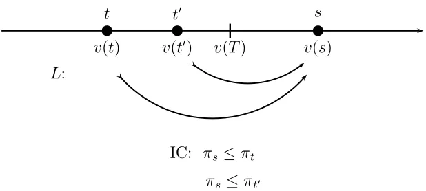
Proposition 4 Assume that there is a type s ∈ T such that: (i) s ∈ L(t)
for every t, and (ii) v(t)< v(T) for every t 6=s. Then the outcome π∗
with
π∗
t =v(T) for all t∈T is the unique optimal mechanism outcome; i.e.,
X
t∈T
ptht(πt)≤
X
t∈T
ptht(π∗t) =hp(v(T))
for every π that is incentive-compatible (i.e., satisfies (IC)), with equality only if πt=π∗t for all t∈T.
Condition (i) says that type s is a “least informative” type (in most examples, this is the type that has no evidence at all); condition (ii) implies, by Lemma 1, that we cannot have v(s) < v(T), and so v(s) is the highest peak: v(t) < v(T) ≤ v(s) for all t 6= s. To get some intuition, consider the simplest case where there are only two types, say,T ={s, t}. The two peaks
v(t) andv(s) satisfyv(t)< v(s),whereas the (IC) constraintπs ≤πt (which
corresponds to s ∈ L(t)) goes in the opposite direction. This implies that the maximum of H(π) = pshs(πs) +ptht(πt) subject to πs ≤ πt is attained
when πs and πt are taken to be equal (ifπs < πt then increasing πs and/or
decreasing πt would bring at least one of them closer to the corresponding
peak, and hence would increase the value of H). Thus πs=πt=xfor some
x, and then the maximum is attained when x equals the peak of hp(x) =
pshs(x) +ptht(x), i.e., when x=v(T).
Proof. Putα:=v(T).We will show that even if we were to consideronly the (IC) constraintsπt≥πs for allt6=sand ignore the other (IC) constraints—
which can only increase the value of the objective function H(π)—the max-imum of H(π) = Pt∈T ptht(πt) is attained when all the πt are equal, and
thus π∗
t =α for all t∈T.
Thus, consider an optimal mechanism outcomeπ0 for this relaxed
prob-lem, and putβ :=π0
s. Since the only constraint onπt fort6=s isπt ≥β,the
fact that ht has its single peak at v(t) implies the following: if β lies before
the peak, i.e., β ≤ v(t), then we must have π0
t = v(t), and if β is after the
peak, i.e., β ≥ v(t), then we must have π0
t =β. Thus,
v(t) v(t′) v(T) v(s)
t t′ s
L:
IC: πs ≤πt
[image:33.595.126.435.149.288.2]πs ≤πt′
Figure 3: Proposition 4
Put T0 :={t∈T :π0
t =β}. We claim that
v(T0)≥α. (8)
Indeed, otherwise v(T0)< α together with v(t)< α for every t /∈T0 (which
holds by assumption (ii) because s ∈ T0 and so t 6= s) would have yielded
v(T) < α by Lemma 1, a contradiction. Now the optimality of π0 implies
thatβ,the common value ofπ0
t for allt ∈T0,must be a (local) maximand of
P
t∈T0ptht(x) (since we can slightly increase or decreaseβ without affecting
the other constraints, namely, πt ≥ πs for all t /∈ T0, which π0 satisfies as
strict inequalities); therefore β equals the single peak of T0, i.e., β =v(T0).
Hence β > v(t) for every t 6= s (by (8) and assumption (ii)), which yields
π0
t =β (by (7)). This shows that T0 (recall its definition) contains allt6=s,
as well as s,and soT0 =T andβ =v(T0) =v(T) =α, completing the proof
that π0
t =α for every t, i.e., π0 =π∗.
Remark. It is not difficult to show directly (that is, without appealing to our Equivalence Theorem) that under the assumptions of Proposition 4 there is a unique truth-leaning equilibrium outcome, namely, the same π∗
with π∗
t = v(T) for all t ∈ T (specifically, the babbling equilibrium (σ, ρ)
(up to replacing some strict inequalities with equalities) identify the case where onecannot separate between the types, whether the principal commits or not.
Proposition 5 Let π∗
∈ RT be the outcome of a truth-leaning equilibrium
(σ, ρ); then π∗
is the unique optimal mechanism outcome.
Proof. By Proposition 2, π∗
t = maxs∈L(t)ρ(s) and ρ(t) = min{π∗t, v(t)} for
every t ∈ T. Thus π∗ satisfies (IC): if t′
∈ L(t) then L(t′)
⊆ L(t) and so
π∗
t′ = maxt′′∈L(t′)ρ(t′′)≤maxt′′∈L(t)ρ(t′′) = π∗t.
We will show H(π∗
) > H(π) for every π 6= π∗
that satisfies (IC). Let
S :={s∈ T :π∗
s =ρ(s)} be the set of messages s in T that are used in the
equilibrium (ρ, σ) (cf. (4) in Proposition 2); and, for every such s ∈ S, let
Ts :={t ∈ T :σ(s|t)> 0} be the set of types that play s. For any π ∈RT,
split the principal’s payoff H(π) as follows:
H(π) = X
t∈T
ptht(πt) =
X
s∈S
¯
σ(s)X
t∈Ts
qt(s)ht(πt) (9)
(recall that, given the strategy σ,we write ¯σ(s) for the probability of s, and
q(s)∈∆(T) for the posterior on T given that s was chosen). Take s ∈ S, and let α :=ρ(s) = π∗
s be the reward there; the principal’s
equilibrium condition (P) implies that
ρ(s) =v(q(s)). (10)
For every t ∈ Ts, t 6= s we have π∗t = ρ(s) (since σ(s|t) > 0), and so t is
unused (since σ(t|t)6= 1) and v(t)< π∗
t (by (5)), and hence
v(t)< v(q(s)) for all t∈Ts, t6=s. (11)
We can thus apply Proposition 4 to the set of types Ts with the distribution
q(s),to get
X
t∈Ts
qt(s)ht(πt)≤
X
t∈Ts
for every π that satisfies (IC), with equality only if πt=π∗t for every t∈Ts.
Multiplying by ¯σ(s) > 0 and summing over s ∈ S yields H(π) ≤ H(π∗
) (use (9) for both π and π∗
) for everyπ that satisfies (IC). Moreover, to get equality we need equality in (12) for each s ∈ S, that is, πt = π∗t for every
t ∈ ∪s∈STs =T,which completes the proof.
4.3
Existence of Truth-Leaning Equilibrium
Here we prove that truth-leaning equilibria exist. The proof uses perturba-tions of the game Γ where a slight advantage is given to revealing the whole truth, both in payoff and in probability. We show that the limit points of Nash equilibria of the perturbed games (existence follows from standard ar-guments) are essentially—up to an inessential modification—truth-leaning equilibria of the original game. See also the discussion in Section 5.4.
Proposition 6 There exists a truth-leaning equilibrium.
Proof. For every 0 < ε < 1 let Γε be the following ε-perturbation of the
game Γ. First, the agent’s payoff is49 x+ε1
s=t when the type is t ∈ T, the
message is s∈T, and the reward isx ∈R; and second, the agent’s strategy
σ is required to satisfy σ(t|t)≥ε for every typet∈T.Thus, first, the agent gets an ε “bonus” in his payoff if he reveals the whole truth, i.e., his type; and second, he must do so with probability at least ε.
A standard argument shows that the game Γε possesses a Nash
equilib-rium. Let Σε be the set of strategies of the agent in Γε; then Σε is a compact
and convex subset of RT×T. Every σ in Σε uniquely determines the
princi-pal’s best reply ρ ≡ ρσ by ρσ(s) = v(q(s)) for every s
∈ T (cf. (P); in Γε
every message is used: ¯σ(s) ≥ εps > 0). The mapping from σ to ρσ is
con-tinuous: the posterior q(s) ∈ ∆(T) is a continuous function of σ (because ¯
σ(s) is bounded away from 0), and v(q) is a continuous function of q (by the Maximum Theorem together with the single-peakedness condition (SP), which gives the uniqueness of the maximizer). The set-valued function Φ that maps each σ ∈ Σε to the set of all σ′
∈ Σε that are best replies to
49