An indoor test methodology for solar powered wireless sensor networks

warwick.ac.uk/lib-publications

Original citation:

Tan, W. M., Sullivan, P., Watson, H., Slota-Newson, J. and Jarvis, Stephen A.. (2016) An indoor test methodology for solar-powered wireless sensor networks. ACM Transactions on Embedded Computing Systems .

Permanent WRAP URL:

http://wrap.warwick.ac.uk/81477

Copyright and reuse:

The Warwick Research Archive Portal (WRAP) makes this work by researchers of the University of Warwick available open access under the following conditions. Copyright © and all moral rights to the version of the paper presented here belong to the individual author(s) and/or other copyright owners. To the extent reasonable and practicable the material made available in WRAP has been checked for eligibility before being made available.

Copies of full items can be used for personal research or study, educational, or not-for profit purposes without prior permission or charge. Provided that the authors, title and full bibliographic details are credited, a hyperlink and/or URL is given for the original metadata page and the content is not changed in any way.

Publisher’s statement:

© ACM, 2016. This is the author's version of the work. It is posted here by permission of ACM for your personal use. Not for redistribution. The definitive version was published in ACM Transactions on Embedded Computing Systems

A note on versions:

The version presented here may differ from the published version or, version of record, if you wish to cite this item you are advised to consult the publisher’s version. Please see the ‘permanent WRAP url’ above for details on accessing the published version and note that access may require a subscription.

Abstract

Repeatable and accurate tests are important when designing hard-ware and algorithms for solar-powered wireless sensor networks (WSNs). Since no two days are exactly alike with regard to energy harvesting, tests must be carried out indoors. Solar simulators are tradition-ally used in replicating the effects of sunlight indoors - however, solar simulators are expensive, have lighting elements that have short life-times, and are usually not designed to carry out the types of tests that hardware and algorithm designers require. As a result, hardware and algorithm designers use tests that are inaccurate and not repeat-able (both for others and also for the designers themselves). In this article we propose an indoor test methodology which does not rely on solar simulators. The test methodology has its basis in astronomy and photovoltaic (PV) cell design. We present a generic design for a test apparatus which can be used in carrying out the test methodol-ogy. We also present a specific design which we use in implementing an actual test apparatus. We test the efficacy of our test apparatus and, to demonstrate the usefulness of the test methodology, perform experiments akin to those required in projects involving solar-powered WSNs. Results of the said tests and experiments demonstrate that the test methodology is an invaluable tool for hardware and algorithm designers working with solar-powered WSNs.

This work is funded in part by theUK Technology Strategy Board (TSB) Emerging Technologies Programme, Project 131187/26835-183208, Keeping the noise down: OPV-based Energy Harvesting Sensors for Urban Noise Pol-lution. Author W. M. Tan is supported in part by the Republic of the Philippines’ Engineering Research and Development for Technology (ERDT) Program.

Authors’ addresses: W. M. Tan, now at the Department of Computer Science, University of the Philippines - Diliman, Quezon City, Metro Manila, Philippines; P. Sullivan, Department of Chemistry, University of Warwick, Coventry, England, United Kingdom; H. Watson and J. Slota-Newson, Polyso-lar Ltd, Hauser Forum, Charles Babbage Road, Cambridge, England, United Kingdom; S. A. Jarvis, Department of Computer Science, University of War-wick, Coventry, England, United Kingdom.

An Indoor Test Methodology for

Solar-powered Wireless Sensor Networks

WILSON M. TAN

, PAUL SULLIVAN

, JOANNA

SLOTA-NEWSON, HAMISH WATSON

, and STEPHEN A.

JARVIS

1

_{Department of Computer Science, University of Warwick,}

Coventry, England, United Kingdom & Department of

Computer Science, University of the Philippines - Diliman,

Quezon City, Metro Manila, Philippines

2

_{Department of Chemistry, University of Warwick, Coventry,}

England, United Kingdom

3

_{Polysolar Ltd., Hauser Forum, Charles Babbage Road,}

Cambridge, England, United Kingdom

4

_{Department of Computer Science, University of Warwick,}

Coventry, England, United Kingdom

September 9, 2016

1

Introduction and motivation

device characteristics. Most tabletop experiments (such as that documented in [12]) utilize actual hardware, but still omit the effects of daylight patterns: as a result, the nodes are possibly exposed to unrealistic conditions that they will never encounter in actual deployments (the ease with which this can be done will be demonstrated later in the article).

Repeatable experiments involving sunlight are also frequently needed in the field of photovoltaic (PV) cell (also called solar cell) design. In this domain, this problem is approached with the help of solar simulators (for example, [24]). Solar simulators generate light that approximates the in-tensity and the spectral content of natural sunlight. Most solar simulators however are designed for single-intensity exposure experiments: they subject the solar cells to a constant specific light intensity. They are not designed to automatically replicate the changing intensity of sunlight throughout the day. The intensity and duration of light to which a solar-powered WSN node is exposed are of primary importance to hardware and algorithm designers: for a given hardware (component sizing) and software (algorithm parame-ters) setup, they determine the system’s performance and survivability - it is therefore important for WSN nodes to be tested with irradiation patterns that mirror real-world conditions. Moreover, solar simulators are expensive and bulky devices, with lighting elements that have very limited lifetimes.

In this work, we present a test methodology which enables repeatable in-door testing of solar-powered WSN nodes without the use of a solar simulator in the test itself. The test methodology induces the solar cell or solar panel to generate a level of power that it will exhibit under outdoor conditions at a specific time and place. The methodology has its basis on insights from PV cell design and astronomy. We firstly present the test methodology in an apparatus-agnostic manner, specifying the general principles of the test ap-paratus design. To prove its practicality however, we present our ownspecific design and implementation of the test apparatus. We present two variant de-signs for the apparatus. The first variant can be used in testing stand-alone wireless sensor network nodes. The second variant is a distributedversion of the first, and can be used as a basis for testbeds designed to test wireless sensornetworks. The performance and accuracy of the test methodology and our test apparatus are verified via a series of experiments. Moreover, we also carry out a series of demonstration experiments, the likes of which will be useful in studies aiming for outdoor deployment of solar-powered WSNs. It must be noted that while this article focuses on WSNs and WSN nodes, the test methodology is also readily applicable to any solar-powered embedded system, even those that are not designed to be networked.

can be used in its implementation; and secondly, the design of an actually-implemented apparatus. We present two variants of the apparatus: central-ized and distributed. We also present the results of two sets of experiments: the first tests the performance of the test apparatus, while the second is com-prised of experiments that demonstrate how the methodology can be used in determining hardware and software parameters for a WSN node.

The remainder of this article is structured as follows. The test methodol-ogy is presented in the following section (Section 2). The design of ageneric test apparatus on which the test methodology can be implemented is pre-sented in Section 3. Section 4 discusses our specific design and implementa-tion of the test apparatus. We test the performance of our test apparatus, and present the results of the said tests in Section 5. The results of two experiments that demonstrate the utility and possible applications of the test methodology are presented in Section 6; limitations are discussed in Sec-tion 7. Related work is discussed in SecSec-tion 8. SecSec-tion 9 presents possible future extensions of the research and concludes the article.

2

Test methodology

Before outlining the general principles of the test methodology we need to understand the relationship between a surface’s irradiance, the surface’s lo-cation, and the current date and time; this will be discussed in Section 2.1. An understanding of a solar cell’s ‘state’ and how such a state can be deter-mined is also required and this will be discussed in Section 2.2. The general principles built from these two examinations are presented in Section 2.3.

2.1

Astronomical model of irradiance

Irradiance (unit W

m2) is the total power from a radiant source falling on a unit

area. A detailed discussion of how irradiance due to the sun is computed at a given location, time of day and time of year, is given in [31] and [15]. In this section, we give a necessarily brief summary of the procedure.

The power density in sunlight which reaches the Earth from the sun is 1,367 W

m2. However, some of this is absorbed in the atmosphere, so the power

density that reaches the surface of the Earth is less. The amount of sunlight absorbed or scattered depends on the length of path through which sunlight has to travel to get to the surface. The path length is generally compared to a path directly vertical to sea level. This path length is designated as 1 atmosphere or AM 1. At AM 1, after absorption is accounted for, the power density is reduced from 1,367 W

m2 to 1,000

W

constant depends only on the air mass, and taking I as the irradiance due to the sun we have Equation 1:

I = 1,367(0.7)AM (1)

However, [30] proposed that a better fit to observed data is obtained through Equation 2:

I = 1,367(0.7)AM0.678

(2)

AM = 1 when the rays from the sun are directly over the surface in consideration. The AM for any ray source direction is given by Equation 3 (all angles stated in this section are in degrees):

AM = 1

cosθz

(3)

where θz is the zenith angle, which is the complement to 90° of the

el-evation α. The elevation is the angle between the sun’s direction and the horizon.

θz = 90−α (4)

The elevation, or α, can be derived from Equation 5:

α=sin−1(sinδsinθ+cosδcosθcosω) (5)

θ is the latitude of the surface. δ is the solar declination, or the angle be-tween the line joining the centres of the Earth and the sun, and the equatorial plane. This can be derived from Equation 6:

δ = 23.45_×sin(360_× n−180

365 ) (6)

wheren is the day in the year (n = 1 on 1st _{January). ω is the angle}

dif-ference between noon and the desired time of day in terms of a 360°rotation in 24 hours:

ω= 12−T

24 ×360 = 15(12−T) (7)

where T is the time of day with respect to solar midnight, on a 24-hour clock.

2.2

Solar cell state

Each solar cell has an associated set of current-voltage (IV) curves (Figure 1). The currently-relevant IV curve is dependent on the irradiance of the solar cell, while the specific point on the curve (the solar cell’s current operat-ing point) is dependent on the electrical load imposed on the solar cell. The currently-relevant IV curve for the solar cell can be determined by measuring the cell’s short circuit current (ISC), which is unique for each level of

irradi-ance. The relationship between the irradiance and the ISC is highly linear

[31]: for instance, if the ISC at 1000 _mW2 is 18.9 mA, the ISC at 500

W m2 will

be approximately 9.45 mA. We can consider the currently-relevant IV curve as the solar cell’s state. It must be noted that how a solar cell is induced to reach a certain state is not relevant here. Two similar cells, exposed to different light sources (different spectral content and intensities) can be said to be state-wise the same, as long as they have the same currently-relevant IV curve. This is the key concept which enables us to replace the lighting element in traditional solar simulators with a relatively low-power, cheaper and more easily-controlled alternative.

0 1 2 3

−5 0 5 10 15 20

Voltage (V)

Curren

t

(mA)

1000W m2

530 W m2

200 W m2

Figure 1: IV curves of a solar panel.

2.3

General principles

We are now in a position to state the general principles of the test method-ology

1. Irradiance for a surface at a certain place, date, and time can be com-puted using the set of equations presented in Section 2.1. Irradiance sequences representing days (or parts of days) can be generated by iteratively solving the set of equations.

be better modeled as a continuous function rather than a discrete se-quence. However, we will be implementing the test methodology using discrete-time systems, so some discretization is necessary. We define the time interval between changes in irradiance values as the temporal resolution of a sequence.

2. The currently-relevant IV curve (hence, the irradiance of the solar cell) can be determined by measuring the solar cell’s ISC. By taking

advan-tage of the linear relationship between theISC and the irradiance level,

an irradiance sequence can therefore be converted to an ISC sequence.

3. The simulation of a day (or part of it) can then be carried out by inducing the solar cell to sequentially produce the ISC values specified

in the ISC sequence.

A single solar cell usually can not produce enough voltage or current to power an application. As such, what are used as energy harvesting devices aresolar panels, which are similar solar cells placed in a series and/or parallel configuration to increase the output voltage and/or current. Like solar cells, solar panels also have IV curves, and their characteristics are derived from that of their component solar cells. Since most devices (including those used in this work) use solar panels and not simply solar cells, we refer to the energy harvesting device in subsequent sections as solar panels.

3

Generic test apparatus design

A generic test apparatus which can carry out the test methodology will need three components.

1. Light source. The light source’s output does not need to have the

same spectral content as sunlight. However, it must coincide (even if not completely) with the frequencies to which the solar panel is sensi-tive. The light source must be able to induce the solar panel to enter states corresponding to different irradiance levels, including the irradi-ance level of 1000 W

m2, also known as 1 sun (the maximum irradiance

due to the sun possible at the surface of the Earth).

2. Current measurement mechanism. A generic test apparatus must

be able to measure the solar panel’s ISC, or a suitable proxy to it.

There are two challenges associated with measuring the ISC - where

The test methodology utilizes ISC for determining the current state

of the solar panel. However, measuring ISC requires that the solar

panel be in a short circuit, which is not the case when it is in a useful configuration (i.e., in a circuit). The problem can be solved by utilizing proxy ISC measurements. Two measurements can serve as proxies for

the ISC: the ISC of a pilot panel, and the output of the panel itself.

We define a pilot panel as solar panel that is of the same type as the solar panel found in the device-under-test (DUT), and co-located with it. Assuming that the two panels have the same characteristics, and are under the same lighting conditions, they will be in the same state (since the currently-relevant IV-curve is defined only by the irradiance of the panel’s surface). TheISC of the pilot panel can then be measured

and used in determining the state of both panels. The schematic of a generic test apparatus which uses the pilot panel ISC as proxy for the

DUT solar panel ISC is shown in Figure 2a.

The actual current of the solar panel can also be used as a proxy to a limited extent. This is due to the current value remaining constant (the same as the ISC) for the most part of an IV curve (Figure 1,

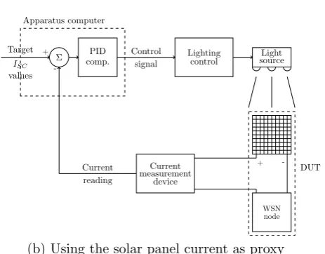
left-side portion). However, depending on the electrical load, this may not always be the case (see right-most part of Figure 1). The schematic of a generic test apparatus which uses the actual solar panel current as proxy for the ISC is shown in Figure 2b.

An additional challenge is the process of measuring the current itself. Accurate current measurement is a complex process. Most microcon-trollers have analog-to-digital converters (ADCs) that measure voltage, but not current. This limits the prospect of the operation being done in distributed systems with low complexity. The current measurement process can be converted to a voltage measurement process with the use of shunt resistors. Shunt resistors however introduce losses, which may be unacceptable when the current is small to begin with. The losses due to a shunt resistor can be minimized by using smaller shunt resistor values. This is made feasible using current sense amplifiers such as the LT6105 [21].

3. Feedback mechanism. A generic test apparatus must have a

feed-back mechanism which will adjust the lighting element’s output in response to the difference between the actual-measured ISC and the

targetISC. A feedback loop can be implemented using a

Target

ISC

values

+ Control

signal

Lighting control PID

comp.

Σ sourceLight

Pilot panel

+

-WSN node Current

measurement device

+

-Current

reading

-Apparatus computer

DUT

(a) Using the pilot panelISC as proxy

Target

ISC

values Σ

-+ PID

comp.

Control signal

Lighting

control sourceLight

Current measurement

device

+ -Current

reading Apparatus computer

DUT

WSN node

(b) Using the solar panel current as proxy

Figure 2: Generic test apparatus design schematic.

unstable system, with the output variable (the ISC in this case) never

converging to a specific value. The performance of the PID controller will also depend on the accuracy of the current measurements.

The design presented above is generic: it is a design which in theory, will enable any type of light source to be used in the apparatus (as long as the spectral content requirements stated above are satisfied). An actual implementation doesnotneed to perfectly conform with the generic design -what is important is that the apparatus is able to induce the solar panel to produce the ISC values contained in the ISC sequence.

4

Test apparatus implementation

We construct two variants of the test apparatus: one for testing WSNnodes, which we call the centralized test apparatus (see Section 4.1), and another that can be used for testing networks of WSN nodes, which we call the distributed test apparatus (see Section 4.2).

4.1

Centralized test system

The lighting element in our implemented test apparatus (both centralized and distributed) is the Luxeon K 8-LED array (LXK8-PW40-0008 [22]). The light intensity of the Luxeon K is current-controlled by the buck regulator-controlled current source LM3406HV [26]. The output of the LM3406HV is then controlled via pulse width modulation (PWM). In the centralized version of our apparatus, the PWM signal is generated by an Arduino Uno [16] (interfaced to a PC via USB cable). In the distributed version, the PWM signal is generated by a TelosB WSN node [35]. For the centralized test apparatus, the Luxeon K is interfaced with a heatsink and mounted on a platform which enables the adjustment of the vertical distance between the LED array and the DUT.

Our choice of components (both for the centralized and the distributed version of our apparatus) is driven by two factors: (1) the availability of components and (2) the size of the DUT’s solar panel (this is particularly important in choosing the light source and designing the adjustable plat-form). As stated in Section 3, a test apparatus can be built from several different types of components, but it must be ensured that the light source can drive the ISC of the DUT’s solar panel to its level at 1 sun. We

ascer-tained that this requirement is met with the use of a sourcemeter (this will be demonstrated later; the result can be seen in Figure 5b).

Figure 3 shows the schematic of our centralized test apparatus; the actual test apparatus is shown in Figure 4.

PC _sequencePWM PWM

signal LM3406 LED

+

-WSN node DUT Arduino

TelosB Power supply unit

Heat sink

Adjustable platform

Solar panel

(a) Lighting element (under the heatsink) and vertically-adjustable stand

Power supply unit

LM3406

Arduino Uno

(b) Arduino and LM3406

Labview

Sourcemeter Base station/

Arduino controller Apparatus (covered)

(c) Test apparatus in operation, with base station and sourcemeter

Figure 4: Centralized test apparatus implementation.

The feedback loop (and its current measurement input) is necessary for dynamically adjusting the lighting element in response to the difference be-tween the measured ISC and the target ISC. This is particularly important

for light sources with resulting ISC values that tend to drift even with a

con-stant light source setting. Some bulbs for example, glow brighter as their filaments heat up, even if the supply voltage remains constant. A feedback loop is not necessary in situations where the resulting ISC for a given lighting

element setting is distinct and unchanging. We call the tendency of a light source to have a distinct and unchanging ISC at each setting its stability.

We note that by ‘light source’ we mean the lighting element along with the mechanism which controls its settings. In our specific setup, the light source is collectively comprised of the LED array, the LM3406HV, and the Arduino. We quantitatively define stability using two metrics. Firstly, we measure the varianceof the solar panelISC observed at a given setting. The variance

provides a measure of how much the ISC fluctuates. The lower the variance,

source has a variance of 0 for all sets of ISC readings. Secondly, we measure

the tendency of the ISC to rise or fall over time using the trendline slope.

Using linear regression, we generate a trendline for the values observed at a given setting, and take note of its slope. This is done for all settings tested. The closer to 0 the trendline slope is, the more stable the light source is at that setting. A perfectly stable light source has a trendline slope of 0 for all sets of ISC readings.

The Arduino allows the user to specify the duty cycle of the PWM signal with 256 values (0 = 0% duty cycle, and 255 = 100% duty cycle). This corresponds to 256 lighting element settings. To test the stability of the light source (vis-`a-vis our recent definition) we test 26 PWM values (multiples of 10, 0 to 250), and measure the resulting solar panel ISC. The vertical

distance between the solar panel and the LED array is set to 60 mm, and the apparatus is covered during the tests to control the lighting. The test is run continuously, with the PWM value increased in a monotonic manner. The

ISC is measured using a Keithley 2401 [19] sourcemeter connected to a PC

running NI Labview [23]. The Labview program collects a current reading every second, resulting in 600 readings per PWM value tested. The measured

ISC values are plotted in Figure 5a. Figure 5b shows the plot of the measured

ISC against the PWM values. Figure 5b is generated by taking the mean of

the 600 current readings taken for each PWM value.

0 50 100 150

·102

0 0.5 1 1.5 2

·10−2

Time (seconds)

ISC

(A)

(a) Plot ofISC as PWM is

monoton-ically increased

0 50 100 150 200 250 0

0.5 1 1.5 2 2.5 ·

10−2

PWM

ISC

(A)

Actual data Modeling function

(b) Plot ofISC vs PWM, both from

averaged empirical data and a linear regression-produced function

Figure 5: Plots for characterizing the solar panel -centralizedtest apparatus configuration.

The variance and trendline slope for each set ofISC readings collected are

the light source is stillhighlystable, exhibiting a maximum variance of 1.825×

10−9 _{(at PWM value 140), and a maximum trendline slope of 2.3×10}−7V s

(at PWM value 140).

0 50 100 150 200 250 0

5 10 15 20

PWM

V

ariance

×10−10

(a) Variance vs PWM

0 50 100 150 200 250 0

1,000 2,000

PWM

T

rendline

slop

e

(

V)s

×10−10

(b) Trendline slope vs PWM

Figure 6: Stability metrics - centralizedtest apparatus.

The extent to which a light source’s stability is acceptable is affected by the temporal resolution of irradiance sequence, or the time interval for which a certain irradiance value holds. A larger interval (poorer temporal resolution) gives more opportunities for the ISC to average out and thus

tolerate more instability. The experiments are carried out utilizing 5-minute intervals (a 24-hour period is divided into 288 sub-periods). This is long enough, we believe, to accommodate the minimal instability of the light source.

We take this opportunity to underscore a point made earlier in the in-troduction about the inadequacy of simple tabletop experiments that do not consult astronomical models. The solar panel we utilize is measured to have a 1 sun ISC of 18.9 mA (some of its IV curves are plotted in Figure 1). The

measurement is done using a calibrated Newport Oriel Sol3A Class AAA 4 x 4 inch solar simulator [24]. As can be seen in Figure 5b however, beyond the PWM value of 210, the ISC already exceeds 18.9 mA. This shows how

easy it is to place the solar panel in a state it will never be in under natural outdoor conditions.

If the light source is stable, ‘day simulation’ will simply consist of se-quentially placing the light source at the appropriate settings. To do this the ISC sequence will have to be converted to a settings sequence which will

then be ‘played’. For our apparatus, the settings sequence is called thePWM sequence.

To convert the ISC sequence to a PWM sequence, we first need to find

be done in several ways. It is desirable that the function complexity be minimized as much as possible without sacrificing too much accuracy. To this end, we adopt a function generated through linear regression (Equation 8):

f(x) = 0.000094738695_×x₋0.000707917246 (8)

Equation 8 is also plotted in Figure 5b. We can then take the inverse of Equation 8, resulting in a current-to-PWM function. By rounding the output of the current-to-PWM function, an ISC sequence can be converted

to a PWM sequence.

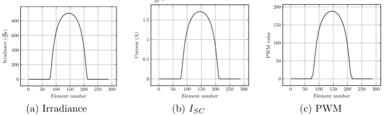
As an example of the transformation between the three types of sequences, Figure 7 shows the irradiance sequence,ISC sequence, and PWM sequence for

September 21 2014 in London, England (coordinates 51.5072°N, 0.1275°W). The astronomical model is evaluated with 5-minute intervals, resulting in a 288-element sequence for the 24-hour period.

0 50 100 150 200 250 300 0

200 400 600 800

Element number

Irradiance

(

W2m

)

(a) Irradiance

0 50 100 150 200 250 300 0

0.5 1 1.5

·10−2

Element number

Curren

t

(A)

(b)ISC

0 50 100 150 200 250 300 0

50 100 150 200

Element number

PWM

value

(c) PWM

Figure 7: Three sequences for September 21 2014 (autumnal equinox), Lon-don.

4.2

Distributed test system

There are some tests for which a single test apparatus will not suffice. For example, a single test apparatus cannot test the effect of differing sunlight patterns within a deployment area on network performance. Such tests are important as deployed nodes will likely receive different sunlight patterns because of several factors, including for example foliage, shadows or cloud cover. To carry out such tests (which are tests on networks, and not simply network nodes), we will need several instances of the test apparatus working together.

cables, and while USB cables are severely limited in length, the power level of the WSN node radios can frequently be adjusted, enabling the implementa-tion of multi-hop networks even within a single room. Nevertheless, this is an unsatisfactory solution as it misses many aspects of actual deployments: for instance, the effect of the environment on topology through wave diffraction, diffusion and refraction.

To this end, we create a version of the test apparatus specifically for testing networks of nodes. Instances of the test apparatus are controlled by a base station, effectively forming a distributed system. Using the original settings sequence as basis, a new sequence can be customized for each test apparatus. To simulate the effect of permanent occlusion such as being under foliage, all the values in the PWM sequence can be attenuated by a certain factor. Temporary occlusion such as temporary cloud cover can be simulated by limiting the attenuation to certain periods. An instance of the test appa-ratus can be located anywhere within a building, as long as it is close to an electrical socket and within communication range of at least one other test apparatus which will enable it to form a multi-hop path to the base station. Our system can be used in constructing an indoor WSN testbed similar to Motelab [38] and Indriya [5], but tailor-made for solar-powered WSNs.

The primary differences between the test apparatus designed for node testing and the test apparatus designed for network testing are in the dis-tribution of the PWM sequence and the generation of the PWM signal. In the test apparatus designed for node testing, PWM signals are generated by an Arduino, which receives the PWM sequence from a PC via a USB cable. In the test apparatus designed for network testing, the PWM signals are generated by a TelosB WSN node, while the PWM sequences are wirelessly received by the same WSN node from the base station. Our base station consists of a PC connected via USB to a TelosB WSN node.

Another difference between the two designs is in the power supply. The centralized version uses a variable-voltage bench power supply, while the distributed version uses a dedicated fixed-voltage power supply unit that is easier to transport. The TelosB WSN node of the distributed test apparatus is currently powered by batteries, although in future design iterations changes will be made so that it can also be powered from the fixed-voltage power supply unit.

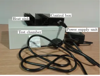
While the test apparatus designed for node testing uses a box cover for keeping out ambient lighting, the distributed test apparatus uses a dedicated test chamber.

[7] implementation of the Dynamic MANET On-demand (DYMO) routing protocol [9]. Dymo is a routing protocol designed by the Internet Engineering Task Force (IETF) to enable dynamic point-to-point routing between mobile nodes. It was originally designed to run on top of the Internet Protocol (IP). The schematic of the distributed test apparatus is shown in Figure 8. Figure 9 shows the actual apparatus.

Base station

TelosB PC

PWM sequence

PWM

signal LM3406 LED

+

-WSN node

DUT/ NUT node TelosB

Distributed test apparatus instance/testbed WSN node

Figure 8: Design schematic of the implemented distributedtest apparatus.

Power supply unit Control box

Test chamber Heat sink

Figure 9: Distributed test apparatus implementation. TelosB and LM3406 inside control box (beside the heatsink).

Note that when using the distributed test apparatus, we effectively end up with two co-located WSNs: one for the test bed/distributed test apparatus (composed of TelosBs in our implementation) and the other the network-under-test (NUT). The members of the NUT (labelled ‘WSN node’ Figure 8) need not be TelosBs. The co-location of two WSNs opens up the possibility of interference, which must be minimized. To achieve this, we employ two measures.

when the patterns are being distributed, and at the end of the simulation, when the nodes report back to the base station. The post-simulation report enables the base station to ascertain that the simulation was successfully carried out by all nodes. We do not deal with the issue of clock drift or clock synchronization in our current implementation.

Secondly, we recommend that the two WSNs use different radio channels or frequency sub-bands. The ability to choose channels is a readily-available feature even in low-power radios such as the CC2420 [27], the radio module used in the TelosB. Additional isolation measures were not felt necessary.

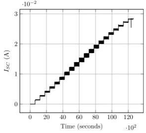
To enable the conversion of ISC sequences to PWM sequences suited to

the distributed test apparatus, we repeat the experiment performed on the centralized test apparatus. The resulting ISC as the PWM duty cycle is

increased is shown in Figure 10a. It should be noted that Figure 10a has differences from Figure 5a. This is to be expected, since the vertical distance between the solar panel and the LED array is different in the two apparatuses (50 mm vs 60 mm). Another difference between the two plots is the range of PWM values. We implement the PWM function of the TelosB using TinyOS’ Alarm mechanism, setting the period of the PWM signal to be 2.04 ms, or the same as that of the Arduino PWM signal. However, unlike in the Arduino where the PWM duty cycle can be specified in 256 levels, in our implementation, one can specify the PWM duty cycle in 2041 levels (0 to 2040, where 0 = 0% duty cycle, and 2040 = 100% duty cycle). We test the PWM values by increments of 100, from 0 to 2000. The results of averaging the ISC values and plotting the averages against the PWM values are shown

in Figure 10b.

0 20 40 60 80 100 120

·102

0 1 2 3

·10−2

Time (seconds)

ISC

(A)

(a) Plot ofISC as PWM is

monoton-ically increased

0 500 1,000 1,500 2,000 0

1 2 3

·10−2

PWM

ISC

(A)

Actual data Modeling function

(b) Plot ofISC vs PWM, both from

averaged empirical data and linear regression-produced function

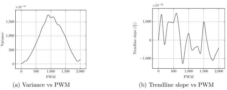
We also plot the variance and trendline slope for each set ofISC readings

collected in Figure 11a and Figure 11b, respectively. The light source of the distributed test apparatus exhibits a maximum variance of 1.74885_×10−7 (at PWM value 900), and a maximum trendline slope of 1.44899×10−7V

s (at

PWM value 600). Similar to the centralized apparatus, the light source of the distributed apparatus is notperfectly stable, but it is sufficiently stable, we believe, for our application.

0 500 1,000 1,500 2,000 0

500 1,000 1,500

PWM

V

ariance

×10−10

(a) Variance vs PWM

0 500 1,000 1,500 2,000

−1,000 0 1,000

PWM

T

rendline

slop

e

(

V)s

×10−10

(b) Trendline slope vs PWM

Figure 11: Stability metrics - distributed test apparatus.

We model the empirical data in Figure 10b using a function generated through linear regression (Equation 9), also plotted in Figure 10b. The inverse of Equation 9 can be used in generating PWM sequences suited for the distributed test apparatus.

f(x) = 0.000014511145_×x₋0.000013327296 (9)

5

Test apparatus performance

The primary purpose of a test apparatus is to induce the solar panel to sequentially produceISC that correspond to the irradiance values determined

by the astronomical model. To test the effectiveness of our test apparatus implementations, we run simulations corresponding to 3 different dates and compare the resulting ISC values to those in the model-generated sequence.

ending just before the beginning of the next day. The same solar panel (1 sun ISC: 18.9 mA) and apparatus setup (DUT-LED array distance: 60 mm

for centralized, 50 mm for distributed) as those used in Section 4 are used. Consequently, the ISC-PWM functions presented in Section 4 are used in

generating the PWM sequences. A Keithley 2401 sourcemeter controlled by Labview measures the short circuit current at 1-second intervals. The readings are averaged over 5-minute sets (300 readings in each set). The averaged readings from the centralized test apparatus, along with the target

ISC values, are shown in Figure 12. We plot the difference between the

theoretical and measured values in Figure 13a.

0 2 4 6 8 10 12 14 ·102

0 0.5 1 1.5 2

·10−2

Time (minutes) Curren t (A) Theoretical Measured

(a) Summer solstice

0 2 4 6 8 10 12 14 ·102

0 0.5 1 1.5 2

·10−2

Time (minutes) Curren t (A) Theoretical Measured

(b) Autumnal equinox

0 2 4 6 8 10 12 14 ·102

0 0.5 1 1.5 2

·10−2

Time (minutes) Curren t (A) Theoretical Measured

(c) Winter solstice

Figure 12: Measured and theoretical (target) ISC values, centralized test

apparatus.

In Figure 12 and Figure 13a it can be seen that the measuredISC values

follow the theoretical ISC values very closely. Between the five minute

aver-ages, thesingle maximum difference between measured value and theoretical value is 0.84 mA for the summer solstice (with a mean of 0.245 mA, 0.36 mA if night portion is excluded), 0.85 mA for the autumnal equinox (with a mean of 0.242 mA, 0.49 mA if night portion is excluded), and 0.789 mA for the winter solstice (with a mean of 0.2 mA, 0.423 mA if night portion is excluded). For all setups, the maximum deviation occurs in the lowest non-zero PWM values - at sunrise or sunset. Referring to Figure 5b (left-side portion), this is to be expected, as this corresponds to the point where the modelling function deviates the most from the empirical data. Another possible source of the deviation is the imperfect stability of the light source. A prominent feature of Figure 12c is the deviation between theoretical and measured ISC in the mid-day section. This can also be explained by the

0 2 4 6 8 10 12 14

·102

0 2 4 6 8

·10−4

Time (minutes)

Theoretical

-measured

difference

(A)

Summer solstice Autumnal equinox

Winter solstice

(a) Centralized apparatus

0 2 4 6 8 10 12 14

·102

0 0.2 0.4 0.6 0.8 1

·10−3

Time (minutes)

Theoretical

-measured

difference

(A)

Summer solstice Autumnal equinox

Winter solstice

(b) Distributed apparatus

Figure 13: Difference between theoretical and measured currents.

for the summer solstice and the autumnal equinox spend significantly less time at the said ISC range compared to the winter solstice sequence, so the

effect is significantly less overall. The precision therefore with which the test apparatus can replicate an ISC sequence closely depends on the values

contained in the sequence. For our specific setup, anISC sequence with more

values that translate to very low non-zero PWM values or are close to 10 mA will tend to be replicated less precisely than those with less.

Before we discuss how the distributed version performs in replicating the ISC sequences, we note that the distributed apparatus cannot properly

inconsistency is caused by the limitations of the TinyOS Alarm, scheduler, or both. To address this limitation (which would lead to significant errors for the apparatus), we round down all values in the PWM sequence that are lower than 50 to 0.

The measuredISC values for the distributed test apparatus are shown in

Figure 14. We also plot the difference between the theoretical and measured values in Figure 13b. The distributed test apparatus is accurate in replicating the sequences for all dates tested. Between the five minute averages, the single maximum difference between measured value and theoretical value is 1.01 mA for the summer solstice (with a mean of 0.155 mA, 0.229 mA if night portion is excluded), 0.585 mA for the autumnal equinox (with a mean of 0.1 mA, 0.218 mA if night portion is excluded), and 0.571 mA for the winter solstice (with a mean of 0.077 mA, 0.156 mA if night portion is excluded). In general, the distributed version outperforms the centralized version when it comes to accuracy. This can be attributed to several factors. The distributed apparatus’ lighting mechanism is superior to that of the centralized apparatus in terms of the trendline slope (although it exhibits greater variance). The distributed apparatus’ modelling function is also a better fit to the data it models. Finally, PWM values in the distributed test apparatus are represented with the range 0-2041, compared to 0-255 in the centralized apparatus. A larger range of numbers translates to greater precision in specifying the PWM signal’s duty cycle.

0 2 4 6 8 10 12 14 ·102

0 0.5 1 1.5 2

·10−2

Time (minutes) Curren t (A) Theoretical Measured

(a) Summer solstice

0 2 4 6 8 10 12 14 ·102

0 0.5 1 1.5 2

·10−2

Time (minutes) Curren t (A) Theoretical Measured

(b) Autumnal equinox

0 2 4 6 8 10 12 14 ·102

0 0.5 1 1.5 2

·10−2

Time (minutes) Curren t (A) Theoretical Measured

(c) Winter solstice

Figure 14: Measured and theoretical (target) ISC values, distributed test

apparatus.

6

Demonstration experiments

deploying solar-powered WSNs. We use the centralized version of the test apparatus in the experiments. The energy harvesting component of our setup is a 30 mm by 30 mm solar panel with ISC of 18.9 mA (the same as that

used in Section 4). The solar panel is connected to a 50 F supercapacitor formed by placing two 100 F Bussmann PowerStor supercapacitors [17] in series (the supercapacitor size is varied in the second experiment). The su-percapacitor is interfaced to a DC-DC converter based on the LT1615 [20]. The DC-DC converter is configured to accept input voltage levels of 1.5 V to 3.0 V, and to output a constant 3.3 V, which is used to power the WSN node. The nodes utilized in this study are TelosB nodes running TinyOS. The application running on the node comprises of a simple sleep-send loop, with the send performed through LowPowerListening [28]. Senders are con-figured to assume the wakeup interval of the receiver as 1-s. All sends are also configured as broadcasts - therefore, at each send, the radio of the node remains active for 1-s before returning to sleep. The interval between the sends is a parameter that is varied in the first experiment. The packets from the node are received by a base station which consists of another TelosB node connected via a USB cable to a netbook. The base station keeps track of packets’ arrival times, and logs the contents of the packets received. The packet has a payload of a single variable which is incremented by the sender node prior to each send. The variable enables us to verify that the node is in continuous operation, and that it has not restarted. The physical setup of the test apparatus is the same as that in Section 4. The three simulated days in Section 4 are also used in the two experiments, but with some mod-ifications. Instead of starting the sequence at midnight (as is the case in the previous experiments), we start the sequence at sunrise. Each experi-ment still runs for 24 hours, therefore the end of each sequence corresponds very closely to the sunrise of the next day. The majority of the experiments involve the measurement of the supercapacitor voltage. For this we utilize a Keithley 2401 sourcemeter connected to a PC running NI Labview. The Labview program takes in a voltage reading every minute.

6.1

Experiment 1: Send interval

volt-age is set to 1.767 V. The results for the summer solstice, autumnal equinox, and winter solstice are shown in Figure 15a, Figure 15b, and Figure 15c, re-spectively. The plots also show the time for the sunset, indicated by a single black vertical line.

0 2 4 6 8 10 12 14 ·102

2 2.5 3 Time (minutes) Sup ercapacitor voltage (V) A B C C*

(a) Summer solstice

0 2 4 6 8 10 12 14 ·102

2 2.5 3 Time (minutes) Sup ercapacitor voltage (V) A B C

(b) Autumnal equinox

0 2 4 6 8 10 12 14 ·102

1 1.5 2 2.5 3 Time (minutes) Sup ercapacitor voltage (V) A B C

(c) Winter solstice

Figure 15: Results for the first experiment. Send interval varied: Setup A, 20-second send interval; Setup B, 40-second send interval; Setup C, 60-second send interval. Initial voltage 2.5 V. 50 F supercapacitor.

From the results it is apparent that a shorter send interval translates to greater energy consumption: this is especially pronounced during nighttime (right of the vertical line) where we see the voltage for Setup A decreasing faster than then voltage for Setup B, which in turn, decreases faster than the voltage for Setup C. The figures also show that there is a peak level to which the supercapacitor voltages can rise. In Figure 15a and Figure 15b, where there are numerous daylight hours, we see the voltages for all setups remaining at the peak level for extended periods of time. In contrast, in Figure 15c the voltage of some setups barely reach the peak before starting to decrease.

In Figure 15a it can be seen that for all setups, the final supercapacitor voltage is higher than the initial. This increase in supercapacitor voltage after a 24-hour period indicates an energy surplus - more energy was har-vested than was spent during the day. As discussed in [11], to ensure energy neutral operation, a daily breakeven or surplus in energy is required: energy neutral operation is the state of an energy harvesting-powered system where it consumes only an amount of energy equivalent to or less than that which it regularly harvests, thus resulting in potentially perpetual operation. Dy-namic power management algorithms can use the increase in voltage level as a cue that the send interval (duty cycle) can be decreased (increased).

(the time between sunrise and sunset) lead to less energy being harvested compared to the summer solstice.

The surplus for Setups B and C persists even in the winter solstice (Fig-ure 15c), although the differences between the final and initial voltages be-come smaller than those during the autumnal equinox. As for Setup A, the final voltage level is lower than the initial level, indicating an energy deficit: a deficit happens when more energy is consumed than harvested during the 24-hour period. A deficit implies that the send interval is not sustainable if consecutive days will display the same pattern, since the energy stored in the energy storage device will progressively get lower. Our experiment results suggest that a send interval of 20-s is too short for our system, especially if the goal is to incur a daily energy surplus or breakeven. Dynamic power management algorithms can take the calculated deficit as a cue to increase (decrease) the send interval (duty cycle).

Setup A in Figure 15c actually exhibits not just a deficit but also a sudden collapse in the supercapacitor voltage which causes the node to stop operat-ing. Continuing the simulation does notcause the node to resume operation indicating the inability of the design to perform cold booting (the process of booting up via energy harvesting while coming from a very low level of charge).

6.2

Experiment 2: Supercapacitor size

In the second experiment, we test how the supercapacitor voltage will evolve under different supercapacitor sizes. This is an example of how hardware parameters can be tested with the test methodology. The node utilized has a send interval of 40 seconds. We test three supercapacitor sizes: 50 F, 33.33 F, and 25 F. We denote the setups with these supercapacitors as Setups A, B, and C, respectively. All supercapacitors are formed by placing two or more 100 F supercapacitors in series.

The energy stored in a capacitor is defined by E = 1

2 ×C×V

2 _whereC

is the size of the capacitor and V is its voltage. For the supercapacitors to have the same initial energy levels, they must have different initial voltages. We choose the values 1.767 V for Setup A, 2.165 V for Setup B, and 2.5 V for Setup C. The initial energy is chosen so that all supercapacitors have initial voltages higher than 1.5 V but lower than 3.0 V, the designed operational limits for the DC-DC converter. The results for the summer solstice, autum-nal equinox, and winter solstice are documented in Figure 16a, Figure 16b, and Figure 16c, respectively.

0 2 4 6 8 10 12 14 ·102

2 2.5 3 Time (minutes) Sup ercapacitor voltage (V) A B C

(a) Summer solstice

0 2 4 6 8 10 12 14 ·102

1.5 2 2.5 3 Time (minutes) Sup ercapacitor voltage (V) A B C

(b) Autumnal equinox

0 2 4 6 8 10 12 14 ·102

1 1.5 2 2.5 3 Time (minutes) Sup ercapacitor voltage (V) A B C

(c) Winter solstice

Figure 16: Plots for the second experiment. Supercapacitor size varied: Setup A, 50 F; Setup B, 33.33 F; Setup C, 25 F. 40-second send interval.

It can be seen in the figures that most setups reach the same peak voltage of around 3.0 V. During days with long charging periods (daylight hours), the supercapacitor voltages remain for an extended period of time at the peak level. An exception is Setup A during the winter solstice (Figure 16c) whose supercapacitor voltage never reaches 3.0 V before starting to decrease. The presence of a common peak voltage has the consequence that the super-capacitors are able to store different amounts of energy.

insufficient for continuous year-long operation: Setup C ends up with a deficit in each day pattern tested, and its supercapacitor voltage collapses during the winter solstice (Figure 16c). We note that increasing the initial voltage will not change the situation since the peak voltage level is already reached by Setup C during the winter solstice. If we assume for simplicity that the peak voltage is attained right before the decrease in voltage due to lack of sunlight, we calculate that Setups A and C consume 113.53 J and 112.01 J respectively during the winter solstice evening. In comparison, Setups C’s peak voltage translates to 114.6 J of stored energy. Given the very small margin, we can deduce that 25 F is too small to store the energy required by the system to operate continuously during the winter solstice evening. We also note that at the point of voltage collapse, Setup C theoretically still has 20.48 J left in stored energy.

The voltage collapse is a system behaviour that will be missed by sim-ulations that employ simplistic models of the energy storage device. Even relatively complex simulators such as PowerTOSSIM [36] only shuts down nodes when the energy storage device contains 0 J - a behaviour clearly not seen in Figure 16c. Examples of studies where the node is shut down only after completely depleting the energy storage device include [14] and [4].

For a software simulator to capture the emergent system behaviour in Figure 16c, the simulator must accurately model not just the energy storage device but also the energy harvesting system, which includes the solar panel and the DC-DC converter (software simulation is discussed in greater detail in Section 8.1). The difficulty of finding a correspondence between a real-world system and a simulation model further highlights the need for a methodology which validates and tests designs at the physical implementation level.

Setup B ends up with a surplus during the summer solstice (Figure 16a) and deficits during the autumnal equinox (Figure 16b) and winter solstice (Figure 16c).

Setup A ends up with a surplus in each of the day patterns tested - this indicates that a 50 F supercapacitorcanstore enough energy that will sustain the system through any night of the year: whether itwillstore enough energy is dependent on the energy it has at the beginning of the day, and the time of year.

energy stored in the device generating the said voltage.

7

Limitations

We recognise that the tests employed in this study are approximations of actual daylight patterns. Weather effects clearly mean that the energy that can be harvested at a specific day, time and place is inherently stochastic. This said, the test methodology that we describe does: (i) provide researchers and hardware/software designers with well-defined limits of the energy con-ditions a node (or network of nodes) may encounter and enables repeatable experiments under these conditions; (ii) provide a framework with which real-world data can be discretised and employed (through Principles 2 and 3 of Section 2.3), should such data exist for a particular region of interest.

Meteorological phenomena can cause the observed irradiation to signif-icantly vary from theoretical values. Irradiance readings are available for some locations. In this study we deliberately chose London, as the London Air Quality Network [18] makes available past irradiation data for some Lon-don boroughs. Other researchers would, therefore, be able to augment this study with additional data should they wish to do so.

Engineers may factor in a test strategy which employs real-world observa-tions before hardware is deployed. In this case we signal two potential pitfalls with this approach: Firstly, open-source irradiance readings are not available for many locations, and data collection would therefore be necessary; Sec-ondly, even if such data were available, understanding the predictability of weather patterns is difficult (as medium- to long-term weather forecasting shows us), and some mathematical modelling would be necessary. It is for these reasons, and the aim for a generic apparatus and methodology, that our work takes the approach that it does.

This test methodology should not be used to compare different solar pan-els. It can however be used for testing (and sizing) different components ‘downstream’ of the solar panel such as the DC-DC converter, the energy storage device, and the microcontroller. For testing different solar panels, a solar simulator must be used. Another advantage of using a solar simulator (assuming that its irradiance can be continuously and automatically varied) is that it will remove the need to derive the ISC vs PWM function, thus

simplifying the test methodology.

panel can be constructed by incorporating features of TempLab [2]. TempLab is an extension for WSN testbeds that allows the control of node temperatures by using infra-red light bulbs and Peltier cooling modules.

8

Related Work

To the best of our knowledge, there are no other studies concerning the indoor testing of solar-powered WSNs without the use of solar simulators. We therefore focus on the test methodologies and power models used in studies concerning solar-powered or energy-harvesting WSNs. We divide such test methodologies into two categories: those that utilize software-based simulations and models (Section 8.1), and those that are used with real-world systems (Section 8.2).

8.1

Software-based simulations and models

8.1.1 Numerical simulations

Most studies on power management algorithms that rely on scheduling tasks (such as [32] and [3]) test their algorithms using numerical simulations with very simple power models. The simulators utilized in these studies are mostly custom-made, and implemented in C or MatLab. The utilization of custom simulators makes experimental comparison and verification difficult. A more significant problem with the test methodology employed in these studies is their sheer simplicity. Hardware non-idealities and the environment are rarely taken into account, therefore, significant work and verification using a methodology suitable for actual devices is required before such algorithms are feasible for actual systems or devices.

8.1.2 Discrete event simulator extensions

An additional approach to simulating the power consumption of energy-harvesting nodes utilizes extensions to existing simulation frameworks. No-table examples of this approach are SensorSim [33] and PowerTOSSIM [36]. PowerTOSSIM [36] is an extension to TOSSIM [13] which enables the simu-lation and measurement of the energy consumption of TinyOS applications. When running a simulation, PowerTOSSIM analyses the instructions in the program and depending on the components utilized by the instruction (and the states the components are in), computes the node power consumption.

exam-ple, a hardware power consumption model is built using microbenchmarks that exercise each hardware component independently. Power consumption readings are taken while microbenchmarks are running in the node. An ex-ample of a tool for power metering of wireless sensor nodes is Quanto [6].

The main drawback of this approach is the difficulty of carrying out hard-ware profiling, and in the case of TOSSIM and PowerTOSSIM, creating an accurate instruction-component model. TinyOS supports several WSN node platforms (Mica [8], Mica2, MicaZ, and TelosB, to mention but a few), but TOSSIM and PowerTOSSIM currently only support the MicaZ platform. An additional drawback is that these simulator extensions only consider the node itself, and not the components usually added to node platforms to en-able them to harvest energy. PowerTOSSIM for instance, does not take into account DC-DC converter efficiency, leakage in the energy storage device, or the environment (sunlight patterns).

8.2

Test methodologies for actual physical systems

Most systems destined for actual deployments are not tested indoors prior to deployment. Instead the energy consumption of the node (in joules per operation, for instance) and the energy that can be harvested from the en-vironment are estimated, and the parameters (such as the application duty cycle) are subsequently set. This approach has obvious drawbacks: the per-formance (and survivability) of the system will depend on the accuracy of the estimates, and such estimates are difficult to acquire with high preci-sion because of factors such as hardware non-idealities and the inherently stochastic nature of the energy that can be harvested from the environment. To compensate, conservative parameters are often used, but this leads to loss of performance and will still not be a guarantee of system survivability.

One such study which employed the ‘estimate-and-deploy’ methodology is described in [37]. They describe an approach used in designing the energy harvesting subsystem of sensor nodes that were used in studying hydrological cycles in forest watersheds. The computations underlying the choice and sizing of components are explained, as well as the rationale for key design decisions. The application that was run on the node is not adaptive: it operated at the same duty cycle, regardless of the environmental conditions. While best effort was made in estimating the parameters, nodes still shut down during the deployment.

Given the lack of calibration, it is very much possible that the energy har-vesting system was induced to produce energy higher than it will under actual outdoor conditions. As we highlighted in Section 4, this is a problem that will lead to poorly-developed systems.

A significant departure from the methods used in most other work, [10] performed experiments (comparison between different energy harvesting WSN node designs) outdoors under natural sunlight: the experiments were done during ‘sunny days in mid-October’ to minimize weather effects. The experi-ments performed, while valid, are impossible to replicate and do not capture seasonal effects.

A drawback with the reliance on actual deployments for testing is that no two day patterns are exactly the same: because of this lack of repeatabil-ity, parameters, algorithms, and designs are difficult to objectively compare. Even if the variability between day patterns is ignored, as in [10], relying on actual deployments means being restricted by one’s location and the current season. For example, to test how the system will perform during winter, the study would have to be performed in winter. A system destined for deployment in the Arctic will have to be tested, at all stages, in the Arctic.

Our test methodology, in comparison, enables the repeatable testing of parameters, algorithms and hardware designs. The studies that result are not limited by the current season or the location where the study is being conducted. How a node (or even network of nodes) will fare in sub-Saharan Africa during winter can be studied in a controlled laboratory experiment.

8.3

Summary and comparison

9

Conclusion and future work

We present an indoor test methodology for solar-powered WSNs. The method-ology is based on astronomical models and PV cell design principles, and it enables repeatable experiments without the need for expensive solar simu-lators. We detail the design of a generic test apparatus which can be used in implementing the test methodology. We also detail the design of our own implemented test apparatus, which has two variants: centralized and distributed. The centralized version can be used in experiments involving isolated solar-powered WSN nodes. The distributed version can be used in testing networks of such nodes. Our implemented designs differ from the generic design in that they do not rely on a feedback loop as a control mech-anism, relying instead on the stability of the light source and a modelling function specifying the relationship between the ISC and the lighting

ele-ment setting. The omission of the feedback loop significantly simplifies the apparatus design.

Our experiments show that the implemented test apparatuses can repli-cate target ISC sequences accurately, although the accuracy varies

depend-ing on the specific ISC value involved. The variations in accuracy between

different ISC values stem from the light source’s imperfect stability and

in-accuracies in the modelling function.

We also perform a series of experiments demonstrating how the test methodology can be used in deriving software and hardware parameters for a WSN node. The results of our experiments largely confirm well-known power management principles. We note however that prior to this work deriving such parameters through repeatable experimentation has been impossible (at least not without a solar simulator).

The study we present is primarily an enablingstudy, and can be applied in many other research areas involving actually-implemented solar-powered WSNs or WSN nodes. For example, it can be used in designing and studying dynamic power management algorithms, or testing the ability of hardware designs to perform cold booting.

Future research can proceed in several directions. Hardware improve-ments can be made: As embedded computing platforms become cheaper, smaller and more powerful, we can integrate greater capability into the test apparatus. For example, measurement of the short-circuit current might, in future variants, be integrated with the apparatus itself (removing the need to derive ISC vs PWM beforehand). Similarly, with smaller and more

found in [34], might also be tested to see whether they are more representa-tive of external conditions. We envisage customised models being created for specific locations and times using historical meteorological data. Any model can theoretically be used, providing their outputs can be converted to anISC

equivalent. Finally, our approach of subjecting nodes to controlled environ-mental conditions to simulate actual energy harvesting, can be applied to energy harvesting WSNs (and WSN nodes) powered by sources other than solar energy, including wind, vibration and ambient radio frequency (RF) energy.

References

[1] Karl Astrom and Tore Hagglund. 1995.PID Controllers: Theory, Design and Tuning (2nd ed.). International Society of Automation (ISA), North Carolina, Chapter 3.

[2] Carlo Alberto Boano, Marco Z´u˜niga, James Brown, Utz Roedig, Chamath Keppitiyagama, and Kay R¨omer. 2014. TempLab: A Testbed Infrastructure to Study the Impact of Temperature on Wireless Sensor Networks. In Proceedings of the 13th International Symposium on In-formation Processing in Sensor Networks (IPSN ’14). IEEE Press, NJ, USA, 95–106. http://dl.acm.org/citation.cfm?id=2602339.2602351

[3] Maryline Chetto and Hui Zhang. 2010. Performance Evaluation of Real-Time Scheduling Heuristics for Energy Harvesting Systems. In Green Computing and Communications (GreenCom), 2010 IEEE/ACM Int’l Conference on Int’l Conference on Cyber, Physical and Social Computing (CPSCom). ACM, New York, NY, USA, 398–403. DOI:

http://dx.doi.org/10.1109/GreenCom-CPSCom.2010.16

[4] Debraj De, Wen-Zhan Song, Shaojie Tang, and Diane Cook. 2012. EAR: An Energy and Activity-Aware Routing Protocol for Wireless Sensor Networks in Smart Environments. Comput. J. (2012). DOI:

http://dx.doi.org/10.1093/comjnl/bxs039

Springer Berlin Heidelberg, New York, NY, USA, 302–316. DOI:

http://dx.doi.org/10.1007/978-3-642-29273-623

[6] Rodrigo Fonseca, Prabal Dutta, Philip Levis, and Ion Stoica. 2008. Quanto: Tracking Energy in Networked Embedded Systems. In Proceed-ings of the 8th USENIX Conference on Operating Systems Design and Implementation (OSDI’08). USENIX Association, Berkeley, CA, USA, 323–338. http://dl.acm.org/citation.cfm?id=1855741.1855764

[7] Jason Hill, Robert Szewczyk, Alec Woo, Seth Hollar, David Culler, and Kristofer Pister. 2000. System architecture directions for net-worked sensors. SIGPLAN Not. 35, 11 (Nov. 2000), 93–104. DOI:

http://dx.doi.org/10.1145/356989.356998

[8] Jason L. Hill and David E. Culler. 2002. Mica: a wireless platform for deeply embedded networks. Micro, IEEE 22, 6 (Nov 2002), 12–24. DOI:

http://dx.doi.org/10.1109/MM.2002.1134340

[9] Internet Engineering Task Force: Mobile Ad hoc Networks Working Group. 2013. Dynamic MANET On-demand (AODVv2) Routing (draft-ietf-manet-dymo-26). (Aug. 2013). Retrieved June 12, 2015 from http://tools.ietf.org/html/draft-ietf-manet-dymo-26

[10] Jaein Jeong, Xiaofan Jiang, and David Culler. 2008. Design and analysis of micro-solar power systems for Wireless Sensor Net-works. In Networked Sensing Systems, 2008. INSS 2008. 5th Inter-national Conference on. IEEE, New York, NY, USA, 181–188. DOI:

http://dx.doi.org/10.1109/INSS.2008.4610922

[11] Aman Kansal, Jason Hsu, Sadaf Zahedi, and Mani B. Srivastava. 2007. Power Management in Energy Harvesting Sensor Networks. ACM Trans. Embed. Comput. Syst. 6, 4, Article 32 (Sept. 2007). DOI:

http://dx.doi.org/10.1145/1274858.1274870

[12] Pius W.Q. Lee, Mingding Han, Hwee-Pink Tan, and Alvin Valera. 2010. An empirical study of harvesting-aware duty cycling in environmentally-powered wireless sensor networks. In Communication Systems (ICCS), 2010 IEEE International Conference on. IEEE, New York, NY, USA, 306–310. DOI:http://dx.doi.org/10.1109/ICCS.2010.5686442

Sensor Systems (SenSys ’03). ACM, New York, NY, USA, 126–137.

DOI:http://dx.doi.org/10.1145/958491.958506

[14] Jun Luo, Jacques Panchard, Micha lPi´orkowski, Matthias Grossglauser, and Jean-Pierre Hubaux. 2006. MobiRoute: Routing Towards a Mo-bile Sink for Improving Lifetime in Sensor Networks. In Proceedings of the Second IEEE International Conference on Distributed Computing in Sensor Systems (DCOSS’06). Springer-Verlag, Berlin, Heidelberg, 480– 497. DOI:http://dx.doi.org/10.1007/1177617829

[15] Tomas Markvart (Ed.). 2000. Solar Electricity (2nd ed.). John Wiley and Sons, England, Chapter 2.

[16] Arduino. 2013. Arduino. (Nov. 2013). Retrieved June 12, 2015 from http://www.arduino.cc/

[17] Cooper Bussmann. 2014. Cooper Bussmann PowerStor superca-pacitors: HV Series. (Jan. 2014). Retrieved June 12, 2015 from http://www.cooperindustries.com/content/dam/public/bussmann/

Electronics/Resources/product-datasheets/Bus Elx DS 4376 HV Series.pdf

[18] Environmental Research Group, King’s College London. 2012. London Air Quality Network. (July 2012). Retrieved September 4, 2015 from http://www.londonair.org.uk/

[19] Keithley Instruments. 2012. 2401 Low Voltage Sourcemeter Instrument.

(Jan. 2012). Retrieved June 12, 2015 from

http://www.keithley.com/data?asset=55849

[20] Linear Technology. 1998. LT1615/LT1615-1: Micropower Step-Up DC/DC Converters in ThinSOT. (March 1998). Retrieved June 12, 2015 from http://cds.linear.com/docs/en/datasheet/16151fas.pdf

[21] Linear Technology. 2013. LT6105: Precision, Extended Input Range Current Sense Amplifier. (Nov. 2013). Retrieved June 12, 2015 from http://cds.linear.com/docs/en/datasheet/6105fa.pdf

[22] Lumileds. 2014. LUXEON K: Plug and play matrix solution with pre-cise flux, Vf and color. (June 2014). Retrieved June 12, 2015 from

http://www.lumileds.com/uploads/366/DS102-pdf

[24] Oriel Instruments. 2012. Oriel Sol3A Class AAA Solar Simulators.

(July 2012). Retrieved June 12, 2015 from

http://assets.newport.com/webDocuments-EN/images/DS-12082Sol3SolarSim.pdf

[25] Texas Instruments. 2009. eZ430-RF2500-SEH: Solar energy harvest-ing development kit. (March 2009). Retrieved June 12, 2015 from http://www.ti.com/lit/ml/sprt506/sprt506.pdf

[26] Texas Instruments. 2013. LM3406: 1.5-A, Constant Current, Buck Reg-ulator for Driving High Power LEDs. (Nov. 2013). Retrieved June 12, 2015 from http://www.ti.com/lit/ds/symlink/lm3406.pdf

[27] Texas Instruments. 2014. CC2420: 2.4 GHz IEEE 802.15.4 / ZigBee-ready RF Transceiver Datasheet. (Oct. 2014). http://www.ti.com/lit/ds/symlink/cc2420.pdf

[28] TinyOS Core Working Group. 2007. TinyOS TEP 105: Low Power Listening. (Nov. 2007). Retrieved June 12, 2015 from http://www.tinyos.net/tinyos-2.x/doc/html/tep105.html

[29] TinyOS Core Working Group. 2008. Tymo. (April 2008). Re-trieved June 12, 2015 from http://tinyos.stanford.edu/tinyos-wiki/index.php/Tymo

[30] Aden B. Meinel and Marjorie P. Meinel. 1976. Applied Solar Energy: An Introduction (1st ed.). Addison-Wesley, Massachusetts, USA.

[31] Roger A. Messenger and Jerry Ventre. 2010. Photovoltaic Systems En-gineering (2nd ed.). CRC Press, Florida, USA, Chapter 2.

[32] Clemens Moser, Davide Brunelli, Lothar Thiele, and Luca Benini. 2006. Real-time scheduling with regenerative energy. In Real-Time Systems, 2006. 18th Euromicro Conference on. IEEE, New York, NY, USA, 260– 270. DOI:http://dx.doi.org/10.1109/ECRTS.2006.23