warwick.ac.uk/lib-publications
Original citation:
Lazic, Ranko and Schmitz, Sylvain (2016) The complexity of coverability in ν-Petri nets. In:
31st Annual ACM/IEEE Symposium on Logic in Computer Science (LICS), New York City, USA,
5–8 Jul 2016. Published in: Proceedings of the 31st Annual ACM/IEEE Symposium on Logic in
Computer Science (LICS)
Permanent WRAP URL:
http://wrap.warwick.ac.uk/79162
Copyright and reuse:
The Warwick Research Archive Portal (WRAP) makes this work by researchers of the
University of Warwick available open access under the following conditions. Copyright ©
and all moral rights to the version of the paper presented here belong to the individual
author(s) and/or other copyright owners. To the extent reasonable and practicable the
material made available in WRAP has been checked for eligibility before being made
available.
Copies of full items can be used for personal research or study, educational, or not-for profit
purposes without prior permission or charge. Provided that the authors, title and full
bibliographic details are credited, a hyperlink and/or URL is given for the original metadata
page and the content is not changed in any way.
Publisher’s statement:
© ACM, 2016. This is the author's version of the work. It is posted here by permission of
ACM for your personal use. Not for redistribution. The definitive version was published in
LICS ’16, July 05 - 08, 2016, New York, NY, USA
Copyright is held by the owner/author(s). Publication rights licensed to ACM.
DOI: http://dx.doi.org/10.1145/2933575.2933593
A note on versions:
The version presented here may differ from the published version or, version of record, if
you wish to cite this item you are advised to consult the publisher’s version. Please see the
‘permanent WRAP url’ above for details on accessing the published version and note that
access may require a subscription.
The Complexity of Coverability in
ν
-Petri Nets
∗
Ranko Lazi´c
DIMAP, Department of Computer Science University of Warwick, UK
lazic@dcs.warwick.ac.uk
Sylvain Schmitz
LSV, ENS Cachan & CNRS & Inria Universit´e Paris-Saclay, France
schmitz@lsv.ens-cachan.fr
Abstract
We show that the coverability problem inν-Petri nets is complete for ‘double Ackermann’ time, thus closing an open complexity gap between an Ackermann lower bound and a hyper-Ackermann upper bound. The coverability problem captures the verification of safety properties in this nominal extension of Petri nets with name management and fresh name creation. Our completeness result establishesν-Petri nets as a model of intermediate power among the formalisms of nets enriched with data, and relies on new algorithmic insights brought by the use of well-quasi-order ideals.
Categories and Subject Descriptors F.2.2 [Analysis of Algorithms
and Problem Complexity]: Nonnumerical Algorithms and Problems
Keywords Well-structured transition system, formal verification, well-quasi-order, order ideal, fast-growing complexity
1.
Introduction
ν-Petri nets (νPN) generalise Petri nets by decorating tokens with data values taken from some infinite countable data domainD. These
values act as pure names: they can only be compared for equality or non-equality upon firing transitions;νPNs have furthermore the ability to createfreshdata values, never encountered before in the history of the computation. Such systems were introduced to model distributed protocols where process identities need to be taken into account (Rosa-Velardo and de Frutos-Escrig 2008, 2011), and form a restricted class of data-centric dynamic systems (Montali and Rivkin 2016). They also coincide with a restriction of theπ-calculus to processes of ‘depth 1’ as defined by Meyer (2008), while their
polyadicextension, which allows to manipulate tuples of tokens, is
equivalent to the fullπ-calculus (Rosa-Velardo and Martos-Salgado 2012)—and Turing-complete.
In spite of their high expressiveness,νPNs fit in the large family of Petri net extensions among thewell-structuredones (Abdulla et al. 2000; Finkel and Schnoebelen 2001). As such, they still enjoy decision procedures for several verification problems, prominently safety (through thecoverabilityproblem) and termination. They share these properties with the other extensions of Petri nets with
∗Work funded in part by the ANR grant ANR-14-CE28-0005
PRODAQ, the EPSRC grant EP/M011801/1, and the Leverhulme Trust Visiting Professor-ship VP1-2014-041.
Permission to make digital or hard copies of all or part of this work for personal or classroom use is granted without fee provided that copies are not made or distributed for profit or commercial advantage and that copies bear this notice and the full citation on the first page. Copyrights for components of this work owned by others than the author(s) must be honored. Abstracting with credit is permitted. To copy otherwise, or republish, to post on servers or to redistribute to lists, requires prior specific permission and/or a fee. Request permissions from Permissions@acm.org.
LICS ’16, July 05 - 08, 2016, New York, NY, USA
Copyright is held by the owner/author(s). Publication rights licensed to ACM. ACM 978-1-4503-4391-6/16/07. . . $15.00
DOI: http://dx.doi.org/10.1145/2933575.2933593
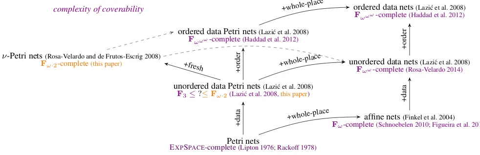
data defined by Lazi´c, Newcomb, Ouaknine, Roscoe, and Worrell (2008), but are something of an intermediate model. Indeed, as shown in Figure 1, they extendunordered Petri data netswith the ability to create fresh data values, but in turn this ability can be simulated (as far as the coverability problem is concerned) by either
ordered data Petri nets—whereDis equipped with a dense linear
ordering—orunordered data nets—where ‘whole-place operations’ allow to transfer, duplicate, or destroy the entire contents of places.
The Power of Well-Structured Systems. This work is part of a general program that aims to understand the expressive power and al-gorithmic complexity of well-structured transition systems (WSTS), for which the complexity of the coverability problem is a natural proxy. Besides the intellectual satisfaction one might find in classi-fying the worst-case complexity of this problem, we hope indeed to gain new insights into the algorithmics of the systems at hand, and into their relative ‘power.’ A difficulty is that the genericbackward
coverabilityalgorithm developed by Abdulla, ˇCer¯ans, Jonsson, and
Tsay (2000) and Finkel and Schnoebelen (2001) to solve coverability in WSTS relies on well-quasi-orders (wqos), for which complexity analysis techniques are not so widely known.
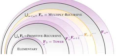
Nevertheless, in a series of recent papers, the exact complexity of coverability for several classes of WSTS has been established. These complexities are expressed using ordinal-indexedfast-growing com-plexity classes(Fα)α (Schmitz 2016), e.g. ‘Tower’ complexity
corresponds to the classF3and is the first non elementary
complex-ity class in this hierarchy, ‘Ackermann’ corresponds toFωand is
the first non primitive-recursive class, ‘hyper-Ackermann’ toFωω and is the first non multiply-recursive class, etc. (see Figure 4). To cite a few of these complexity results, coverability isFω-complete
for reset Petri nets and affine nets (Schnoebelen 2010; Figueira et al. 2011),Fωω-complete for lossy channel systems (Chambart and Schnoebelen 2008; Schmitz and Schnoebelen 2011) and unordered data nets (Rosa-Velardo 2014), and even higher complexities appear for timed-arc Petri nets and ordered data Petri nets (Fωωω-complete, see Haddad et al. 2012) and priority channel systems and nested counter systems (Fε0-complete, see Haase et al. 2014; Decker and
Thoma 2016); see the complexities in violet in Figure 1 for the Petri net extensions related toνPNs.
All those results rely on the same general template (see Schmitz and Schnoebelen 2013, for a gentle introduction):
1. for the upper bound, acontrolled bad sequencecan be extracted from any run of the backward coverability algorithm, and in turn the length of this sequence can be bounded using alength
function theoremfor the wqo at hand (e.g., Cicho´n and Tahhan
Bittar 1998; Figueira et al. 2011; Schmitz and Schnoebelen 2011; Rosa-Velardo 2014, for the mentioned results);
ordered data Petri nets(Lazi´c et al. 2008) Fωωω-complete(Haddad et al. 2012)
complexity of coverability ordered data nets(Lazi´c et al. 2008)
Fωωω-complete(Haddad et al. 2012)
ν-Petri nets(Rosa-Velardo and de Frutos-Escrig 2008)
Fω·2-complete(this paper) unordered data nets(Lazi´c et al. 2008)
Fωω-complete(Rosa-Velardo 2014)
affine nets(Finkel et al. 2004)
Fω-complete(Schnoebelen 2010; Figueira et al. 2011)
unordered data Petri nets(Lazi´c et al. 2008) F3≤?≤Fω·2(Lazi´c et al. 2008,this paper)
Petri nets
EXPSPACE-complete(Lipton 1976; Rackoff 1978)
+whole-place
+order
+order
+fresh +whole-place
+data
[image:3.612.55.546.78.237.2]+data +whole-place
Figure 1. A short taxonomy of some data enrichements of Petri nets. Complexities in violet refer to the already known complexities for the coverability problem; the exact complexity in unordered data Petri nets is unknown at the moment. As indicated by the dashed arrows, freshness can be enforced using a dense linear order or whole-place operations.
Contributions. In this paper, we pinpoint the complexity of cov-erability inνPNs by showing that it is complete forFω·2, i.e. for
‘double Ackermann’ complexity. This solves an open problem: the best known lower bound wasFω, from a reduction from coverability
in reset Petri nets (Rosa-Velardo and de Frutos-Escrig 2011), while the best known upper bound wasFωωfrom the more general case of unordered data nets (Rosa-Velardo 2014), leaving a considerable complexity gap.
We believe thisFω·2-completeness is remarkable on two counts.
First, this is the first instance of a ‘natural’ decision problem com-plete for an intermediate complexity class between Ackermann and hyper-Ackermann. Second, the usual template for such complexity results, summed up in points 1 and 2 above,failsforνPNs, in the sense that all it could prove are the aforementionedFωlower bound
andFωωupper bound. As a result, we had to design new techniques, which we think are of independent interest.
These new techniques are inspired by another case where the template in 1 and 2 fails, namely that of Petri nets. Indeed, cover-ability in Petri nets is EXPSPACE-complete, as shown by Rackoff (1978) for the upper bound and by Lipton (1976) for the lower bound. These results however do not rely on wqos and are quite specific to Petri nets, and their generalisation to a formalism as rich asνPNs required new insights:
•For the upper bound, we analyse the complexity of the back-ward coverability algorithm when seen dually as computing a decreasing sequence ofdownwards-closedsets. Such sets can be represented as finite unions ofideals(Bonnet 1975; Finkel and Goubault-Larrecq 2009); see Section 3.
We have recently shown that, for Petri nets, this dual view allows to exhibit an invariant on the ideals appearing during the course of the execution of the backward coverability algorithm, which in turn yields a dramatic improvement on its complexity analysis from Fω to 2EXPTIME (Lazi´c and Schmitz 2015). The same bound had already been established by Bozzelli and Ganty (2011) using Rackoff’s analysis, but this new viewpoint is applicable to any WSTS with effective ideal representations, and enables us to proceed along similar lines in Section 4 and to obtain the desiredFω·2upper bound.
•For the lower bound, we follow the pattern of Lipton’s proof, in that we design an ‘object-oriented’ implementation of the double Ackermann function inνPNs. By this, we mean that the implementation provides an interface with increment, decrement,
zero, and max operations on larger and largercountersup to a double Ackermannian value. This allows then the simulation of a Minsky machine working in double Ackermann space and establishes the matchingFω·2lower bound.
The basic building blocks of this development are Ackermannian counters reminiscent of the construction of Schnoebelen (2010) for reset Petri nets. The catch is that we need to be able to mimick this construction for non-fixed dimensions and to combine it with an iteration operator—of the kind employed recently by Lazi´c et al. (2016) in the context of channel systems with insertion errors to show Ackermann-hardness—, which led us to develop delicate indexing mechanisms by data values; see Section 5.
We assume the reader is already familiar with the basics of Petri nets, and start with the formal definition ofνPNs and of their seman-tics in the upcoming Section 2. Due to space constraints, some tech-nical material and proofs will be found in the full version of the pa-per, available fromhttps://hal.inria.fr/hal-01265302/.
2.
ν
-Petri Nets
We define the syntax ofνPNs exactly like Rosa-Velardo and Martos-Salgado (2012). Their semantics can be stated in terms of finitely supported partial maps from an infinite data domainDto markings
inNP, telling for each data value how many tokens with that value appear in each place. However, we find it easier to work with a slightly more abstract but equivalentmultiset semantics, which accounts for the fact that the semantics is invariant under permutations of the data domainD, and eschews any explicit
reference to this data domain; see Section 2.2. Following Rosa-Velardo and Martos-Salgado (2012), we also illustrate the expressive power ofνPNs in Section 2.3 by showing how they can implement reset Petri nets.
2.1 Finite Multisets
LetAbe a set. Consider thecommutationequivalence∼over finite sequences inA∗: this is the transitive reflexive closure∼def
=∼∗
1of
the relation∼1 defined byuabv ∼1 ubavfor allu, v ∈A∗and
a, b∈A. We define (finite)multisetsas∼-equivalence classes of
A∗, and writeA⍟ def
=A∗/∼for the set of multisets overA. We manipulate a multiset through any of its representatives in
p0
p1
p2
t
xxy
y x
xν
Fx: 2
Fy:
[image:4.612.60.290.71.118.2]Fν:
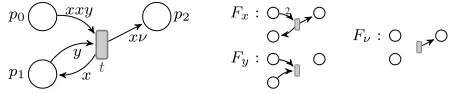
Figure 2. AνPN and the associated flows ofx,y, andν.
multiset. Note that this viewpoint matches the definition of a finite multiset as afinitely supportedfunctionm:A→N, i.e. such that its
supportSupp(m)def
={a∈A|m(a)6= 0}is finite. For instance, Supp([aab]) ={a, b}and[aab](a) = 2and[aab](b) = 1. The
length |m| of a multisetm is the length of any representative
and satisfies|m| = P
a∈Am(a) =
P
a∈Supp(m)m(a) in the
functional view.
Sums. Given two multisetsmandm0over a setA, theirsum(also called theirunion)m⊕m0is represented by the concatenation of their representatives. From the functional viewpoint,(m⊕m0)(a) =
m(a) +m0(a)for alla∈A, with length|m⊕m0|=|m|+|m0| and supportSupp(m⊕m0) =Supp(m)∪Supp(m0).
Embeddings. Assume (A,≤A) is a quasi-order (qo), i.e. that Ais equipped with a reflexive transitive relation≤A ⊆A×A.
Anembeddingfrom a multisetm = [a1· · ·a|m|]into a multiset
m0 = [a01· · ·a0|m0|]is an injective functione:{1, . . . ,|m|} →
{1, . . . ,|m0|} such that ai ≤A a0e(i) for all 1 ≤ i ≤ |m|.
Given such an e, we can decompose m0 in a unique manner as m00 ⊕[a0e(1)· · ·a
0
e(|m|)] for somem
00
. Note that in general
m6= [a0e(1)· · ·a
0
e(|m|)], unless≤Ais the equality relation overA.
We say thatm0embedsmand writemvm0if there exists an embeddingefrommtom0; observe that(A⍟
,v)is also a qo.
Markings. Let(P,=)be a finite set ordered by equality. We call a vectorm∈NP amarking. Markings can be added pointwise by (m+m0)(p) def
=m(p) +m0(p)for allp∈P, and compared using
theproduct orderingm≤m0, holding iffm(p)≤m0(p)for all
p∈P. Note that(NP,+,≤)is isomorphic to(P⍟,⊕,v), but we
shall use the former to avoid confusion with other multisets.
2.2 Syntax and Semantics
LetX andΥbe two disjoint infinite countable sets ofnon-fresh
variablesandfresh variablesrespectively, and letVars def
=X ]Υ.
Syntax. Aν-Petri netis a tupleN =hP, T, FiwherePis a finite non-empty set ofplaces,Tis a finite set oftransitionsdisjoint from
P, andF: (P×T)∪(T×P)→Vars⍟
is aflowfunction. For any transitiont∈T, letInVars(t)def
=S
p∈PSupp(F(p, t))
andOutVars(t) def
=S
p∈PSupp(F(t, p))denote its sets of input
and output variables respectively, andVars(t) def
= InVars(t)∪ OutVars(t); we require that
1. fresh variables are never input variables:Υ∩InVars(t) =∅,
2. all the non-fresh output variables are also input variables: OutVars(t)∩ X ⊆InVars(t).
WritingX(t)def
=Vars(t)∩ XandΥ(t) def
=Vars(t)∩Υ, this entails X(t) =InVars(t)andΥ(t) =OutVars(t)∩Υ.
For a variablex∈Vars, theflow ofxis the functionFx: (P× T)∪ (T ×P) → N defined by Fx(p, t)
def
= F(p, t)(x) and
Fx(t, p) def
= F(t, p)(x). When we fix a transition t ∈ T, we seeFx(P, t)andFx(t, P)as markings inNP. Intuitively, aνPN
synchronises a potentially infinite number of Petri nets acting on the same places and transitions. See Figure 2 for a depiction; as usual with Petri nets, places are represented by circles, transitions by rectangles, and non-null flows by arrows labelled with their values.
We define thesizeof aνPN as|N|def
= max(|P|,|T|,P
p,t|F(p, t)|+
|F(t, p)|)(this corresponds to a unary encoding of the coefficients in the multisets defined byF).
Multiset Semantics. AνPN defines an infinite transition system hConfs,−→iwhereConfs def
= (NP) ⍟
is the set ofconfigurations and−→ ⊆Confs×Confsis called thesteprelation.
Let us associate with any transitiont ∈ T two multisets of markings, in(NP)
⍟
, of inputs and fresh outputs respectively:
in(t) def
=M
x∈X(t)
[Fx(P, t)], outΥ(t)
def
=M
ν∈Υ(t)
[Fν(t, P)]. (1)
Given a configurationM = [m1· · ·m|M|], we say thattisfireable
fromMif there exists an embedding fromin(t)intoM, which here can be seen as an injective functione:X(t)→ {1, . . . ,|M|}with
Fx(P, t)≤me(x)for allx∈ X(t). We call such aneamodefort
andM; giventandMthere are finitely many different modes.
A modeefortandMdefines a step: it uniquely determines two configurationsM0andM00such that
M=M00⊕M
x∈X(t)
[me(x)], (2)
M0=M00⊕outΥ(t)⊕M
x∈X(t)
[m0e(x)], (3)
where for allx∈ X(t),m0e(x) def
=me(x)−Fx(P, t) +Fx(t, P).
We writeM −e,t−→M0in such a case. We write as usualM−→t M0
if there existsefortandMsuch thatM −e,t−→M0, andM−→M0
if there existst ∈ T such thatM −→t M0. In other words, the transitiont:
• appliesFxfor each non-fresh variablex∈ X(t)to a different
individual markingme(x)≥Fx(P, t)ofM, replacing it with
the markingm0e(x),
• leaves the remaining markings inM00untouched, and • furthermore adds new markingsFν(t, P)for each fresh variable
ν∈Υ(t)to the resulting configuration.
Example 1. Consider the transitiontin Figure 2 acting onP = {p0, p1, p2}and a configurationM = [m1m2m3]wherem1=
(2,1,1),m2= (2,0,0), andm3= (1,1,0).
We have in(t) = [(2,0,0)(1,1,0)] and outΥ(t) = [m4]
with m4 = (0,0,1), and three possible modes. We can have
e1(x) = m1, resulting inm01 = (0,2,2), ande1(y) = m3,
resulting in m03 = (0,0,0), hence M
e1,t
−−→ [m01m2m03m4].
Another possibility is to havee2(x) =m2yieldingm02= (0,1,1)
ande2(y) =m1yieldingm001 = (1,0,1), showing thatM
e2,t
−−→ [m001m02m3m4], and a last possibility is to havee3(x) =m2and
e3(y) =m3, resulting in a stepM
e3,t
−−→[m1m02m
0
3m4].
2.3 Example: Reset Petri Nets
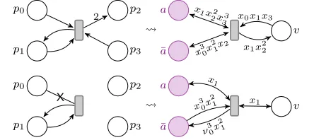
Rosa-Velardo and Martos-Salgado (2012) show thatνPNs are able to simulatereset Petri nets, an extension of Petri nets with special arcs that empty a place upon firing a transition. A remarkable aspect of the construction we are going to sketch here is that three places and a simple addressing mechanism are enough to simulate reset Petri nets with an arbitrary number of places—recall that the latter have an Ackermannian-hard coverability problem (Schnoebelen 2010). This explains why we will be able to push the lower bound beyond Ackermann-hardness in Section 5, where we design more involved addressing mechanisms.
Given any reset Petri net with placesP={p0, . . . , pn−1}, we
p0
p1
p2
p3
2 a
¯
a
v x1x2
2x33
x30x 2
1x2
x0x1x3
x1x22
p0
p1
p2
p3
X
a
¯
a
v
ν30x 2
1
x1
x30x 2
[image:5.612.63.285.72.171.2]1 x1
Figure 3. Examples of simulations of reset Petri net transitions (left) by aνPN (right).
and¯ato maintain anaddressingmechanism for the original places inP, whilevmaintains the actual token counts of the original net. The placesaand¯ausendifferent data values, each with distinct counts of tokens; more precisely, all the reachable configurations
M are of the form[m0· · ·mn−1]⊕M0 wheremi(a) =iand mi(¯a) =n−1−ifor all0 ≤i < n, and all the markingsm
inM0areinactive, i.e. withm(a) +m(¯a)< n−1. Each active
markingmisimulates the placepiof the original net by holding in mi(v)the number of tokens in placepi.
For instance, the top of Figure 3 shows how a transition of a Petri net with4places (on the left) can be simulated with this construction (on the right). The flows of each variablex0, x1, x2, x3with places
aand¯aidentify uniquely the placesp0, p1, p2, p3of the original net,
while the flows with placevupdate the token counts accordingly. The interest of this addressing mechanism is that it allows to simulate reset transitions, like the one on the bottom left of Figure 3 that empties placep0upon firing. This is performed by creating a
fresh markingm00withm
0
0(a) = 0,m
0
0(¯a) = 3, andm
0
0(v) = 0;
after the transition step, we will havem0(a) =m0(¯a) = 0and
m0might still have some leftover tokens inv, but it is inactive and
will be ignored in the remainder of the computation.
3.
Backward Coverability
The decision problem we are interested in iscoverability:
input:aνPN, and two configurationsM0, M1
question:does there existM wM1such thatM0−→∗M?
We instantiate in this section the backward coverability algorithm from (Lazi´c and Schmitz 2015) for νPNs. This algorithm is a dual of the classical algorithm of Abdulla et al. (2000) and Finkel and Schnoebelen (2001): instead of building an increasing chain
U0 (U1 (· · · of upwards-closed setsUkof configurations that
can cover the targetM1 in at mostksteps, it constructs instead
a decreasing chainD0 ) D1 ) · · · of downwards-closed sets Dk of configurations thatcannot cover the target ink or fewer
steps (see Section 3.3). Like the usual backward algorithm, the termination and correctness of this dual version hinges on the fact thathConfs,−→,viis a WSTS (see Section 3.1). We need however an additional ingredient, which is a means of effectively representing and computing our downwards-closed setsDkof configurations.
We rely for this onidealsof(Confs,v), which play the same role as finite bases in the classical algorithm; see Section 3.2.
3.1 ν-Petri Nets are Well-Structured
Well-Quasi-Orders. Let(A,≤A)be a qo. Given a setS ⊆ A,
itsdownward-closureis↓S def
= {a ∈ A | ∃s ∈ S . a ≤A s};
whenSis a singleton{s}we write more simply↓s. A setD⊆Ais
downwards-closed(also calledinitial) if↓D=D. Upward-closures
↑Sand upwards-closed subsets↑U =U are defined similarly.
Awell-quasi-order (wqo) is a qo(A,≤A) where everybad
sequencea0, a1, . . . of elements overA, i.e. withai 6≤A ajfor
alli < j, is finite (Higman 1952). Equivalently, it is a qo with
thedescending chain property: all the chainsD0)D1 )· · · of
downwards-closed subsetsDj⊆Aare finite. Equivalently, it has
thefinite basis property: any non-empty subsetS⊆Ahas a finite
number of minimal elements (and at least one minimal element) up to equivalence.
For instance, any finite setP equipped with equality forms a wqo(P,=): its downwards-closed subsets are singletons{p}for
p∈ P, and its chains of downwards-closed sets are of length at most one. Assuming(A,≤A)is a wqo, then finite multisets overA
provide another instance:(A⍟
,v)is also a wqo as a consequence of Higman’s Lemma. Hence both the sets of markings(NP,≤)and
of configurations(Confs,v)of aνPN are wqos.
Compatibility. The transition systemhConfs,−→idefined by a
νPN further satisfies acompatibilitycondition with the embedding relation: ifM1vM10andM1−→M2, then there existsM20wM2
withM10 → M
0
2. In other words,vis a simulation relation on
the transition systemhConfs,−→i. Since(Confs,v)is a wqo, this transition system is thereforewell-structured(Abdulla et al. 2000; Finkel and Schnoebelen 2001).
3.2 Effective Ideal Representations
Ideals. Let(A,≤A)be a wqo. AnidealIofAis a non-empty,
downwards-closed, and (up-)directedsubset ofA; this last condition enforces that, ifa, a0are inI, then there existsb∈Ithat dominates both:a≤Abanda0≤Ab. For example, looking again at the case
of finite sets(P,=), we can see that singletons{p}are ideals. In fact, more generally↓afora∈Ais always an ideal ofA. But there can be other ideals, e.g.I⍟
is an ideal ofA⍟
ifIis an ideal ofA. The key property of wqo ideals is that any downwards-closed setDover a wqo has a uniquedecompositionas a finite union
D=I1∪ · · · ∪In, where theIj’s are incomparable for inclusion—
this was shown e.g. by Bonnet (1975), and by Finkel and Goubault-Larrecq (2009) in the context of complete WSTS (and generalised to Noetherian topologies). Ideals are alsoirreducible: ifI⊆D1∪D2
for two downwards-closed sets D1 and D2, then I ⊆ D1 or
I⊆D2.
Effective Representations. Although ideals provide finite decom-positions for downwards-closed sets, they are themselves usually infinite, and some additional effectiveness assumptions are neces-sary to employ them in algorithms. In this paper, we will say that a wqo(A,≤A)haseffectiveideal representations (see Finkel and
Goubault-Larrecq 2009; Goubault-Larrecq et al. 2016, for more stringent requisites) if every ideal can be represented, and there are algorithms on those representations:
(CI)to checkI⊆I0for two idealsIandI0,
(II)to compute the ideal decomposition ofI∩I0for two idealsI
andI0,
(CU’)to compute the ideal decomposition of the residualA\ ↑a= {a0∈A|a6≤Aa0}for anyainA.
All these effectiveness assumptions are true of the representations for(NP,≤)and(Confs,v)described by Goubault-Larrecq et al.
(2016), which we recall next.
Extended Markings. LetNω =def N] {ω}, where ‘ω’ denotes a
new top element withω+n=ω−n=ω > nfor alln∈N. An
extended markingis a vectore∈NPω. The product ordering and
pointwise sum operations are lifted accordingly. Then the ideals of (NP,≤)are exactly the sets
JeK def
defined by extended markingse∈NPω. Note thatNPωcontainsNP
as a substructure. Regarding effectiveness assumptions, let us just mention that, for (CI),JeK⊆Je
0
Kiffe≤e
0
. See (Goubault-Larrecq et al. 2016) for more details.
Extended Configurations. Note that, since (NP
ω,≤) is a qo,
((NPω) ⍟
,v)is also a qo—they are in fact both wqos. Anextended
configurationis a pair(B, S) comprising a finitebasemultiset
B ∈ (NPω) ⍟
and a finite starset S ⊆ NPω. Then the ideals of
(Confs,v)are exactly the sets
JB, SK def
={M ∈Confs| ∃E∈S⍟
. M vB⊕E} (5)
defined by extended configurations.
This representation is however not canonical, in the sense that there can be(B, S) 6= (B0, S0) with JB, SK = JB0, S0K. For instance, ife≥e0, then for all extended configurations(B, S),
JB, S∪ {e,e
0
}K=JB, S∪ {e}K, (6)
JB⊕[e
0
], S∪ {e}K=JB, S∪ {e}K. (7)
In fact, those are the only two situations, and reading equations (6) and (7) left-to-right asreduction rules—which are furthermore confluent—we can associate to any extended configuration(B, S) a uniquereducedextended configuration. Such an extended config-uration(B, S)is such thatSis an antichain and, for all extended markingse∈Sande0 ∈Supp(B),e6≥e0. Reduced extended configurations provide canonical representatives for the ideals of (Confs,v); we writeXConfsfor the set of all reduced extended configurations. In the following, for an idealIof(Confs,v)we write(B(I), S(I))for its canonical representative inXConfs.
Observe that XConfs also embeds Confs as an isomorphic substructure: any configurationMcan be associated to the extended configuration(M,∅).
Regarding effectiveness assumptions, we shall only comment on (CI) and refer the reader to (Goubault-Larrecq et al. 2016) for details. Given two reduced extended configurations(B, S)and(B0, S0)in XConfs,JB, SK⊆JB
0
, S0Kiff∃E∈S0⍟
such thatBvB0⊕E, andS⊆HS0, where ‘⊆H’ denotes theHoareordering:S⊆HS0
iff for alle∈Sthere existse0∈S0such thate≤e0.
3.3 Backward Coverability Algorithm
Consider aνPN and a target configurationM1. Define
D∗=def{M∈Confs| ∀M0wM1. M→
∗
M0} (8)
as the set of configurations that do not coverM1. The purpose of
the backward coverability algorithm is to computeD∗; solving a
coverability instance with source configurationM0then amounts to
checking whetherM0belongs toD∗.
Let us define the reachability relation in at mostk ∈Nsteps
by→≤0 def
= {(M, M) | M ∈ Confs}and→≤k+1 def
= →≤k∪
{(M, M00)| ∃M0 ∈Confs. M →M0→≤k
M00}. The idea of the algorithm is to compute successively for everykthe setDkof
configurations that donotcoverM1inkor fewer steps:
Dk def
={M∈Confs| ∀M0wM1. M→
≤k
M0}. (9)
As shown in (Lazi´c and Schmitz 2015, Claim 3.2) these over-approximationsDkcan be computed inductively onk:
D0=Confs\ ↑M1, Dk+1=Dk∩Pre∀(Dk), (10)
where for any setS⊆Confsits set ofuniversal predecessorsis
Pre∀(S)=def{M ∈Confs| ∀M0.(M→M0⇒M0∈S)}. (11)
This set is downwards-closed ifSis downwards-closed (Lazi´c and Schmitz 2015, Claim 3.3). We need here to check an additional effectiveness assumption forνPNs (which holds, see the full paper):
(Pre)the ideal decomposition ofPre∀(D)is computable for all
downwards-closedD,
whereDis given as a finite set of ideal representations. ThenD0
is computed using (CU’), and at each iteration the intersection of Pre∀(Dk)withDkis also computable by (Pre) and (II).
The algorithm terminates as soon asDk ⊆ Dk+1, and then
Dk+j=Dk=D∗for allj. This is guaranteed to arise eventually
by the descending chain condition, since otherwise we would have an infinite descending chain of downwards-closed setsD0)D1) D2)· · ·. The termination checkDk⊆Dk+1is effective by (CI):
by ideal irreducibility,Dk=I1∪ · · · ∪In⊆J1∪ · · · ∪Jr =Dk+1
for idealsI1, . . . , Inand idealsJ1, . . . , Jmif and only if for all
1≤i≤nthere exists1≤j≤rsuch thatIi⊆Jj.
4.
Complexity Upper Bounds
We establish in this section a double Ackermann upper bound on the complexity of coverability inνPNs. The main ingredient to that end is a combinatorial statement on the length ofcontrolleddescending chains of downwards-closed sets, and we define in Section 4.2 control functions and exhibit a control on the descending chain
D0 ) D1 ) · · · built by the backward coverability algorithm
for aνPN. One can extract a controlled bad sequence from such a controlled descending chain (see Section 4.3), from which the
length function theorem of Rosa-Velardo (2014) yields in turn
an hyper-Ackermann upper bound. In order to obtain the desired double Ackermann upper bound, we need to refine this analysis. We observe in Section 4.4 that the descending chains forνPNs enjoy an additionalstar monotonicityproperty. This in turn allows to prove the upper bound by extracting Ackermann-controlled bad sequences of extended markings; see Theorem 9. The final step is to put this upper bound in the complexity classFω·2.
4.1 Fast-Growing Complexity Classes
In order to express the non-elementary functions required for our complexity statements, we employ a family of subrecursive functions (hα)α indexed by ordinals α known as the Cicho´n
hierarchy (Cicho´n and Tahhan Bittar 1998).
Ordinal Terms. We use ordinal termsαinCantor Normal Form (CNF), which can be written as termsα = ωα1 +· · ·+ωαn whereα1≥ · · · ≥αnare themselves written in CNF. Using such
notations, we can express any ordinal belowε0, the minimal fixpoint
ofx =ωx. The ordinal0is obtained whenn = 0; otherwise if αn= 0the ordinalαis asuccessorordinalωα1+· · ·+ωαn−1+ 1,
and ifαn > 0the ordinalαis alimitordinal. We usually write
‘λ’ to denote limit ordinals; any such limit ordinal can be written uniquely asγ+ωβwithβ >0.
Fundamental Sequences. For all xinNand limit ordinalsλ,
we use a standard assignment offundamental sequencesλ(0)< λ(1)<· · · < λ(x)<· · · < λwith supremumλ. Fundamental sequences are defined by transfinite induction by:
(γ+ωβ+1)(x) def
=γ+ωβ·(x+ 1), (γ+ωλ)(x)def
=γ+ωλ(x).
For instance,ω(x) =x+ 1,ω2(x) =ω·(x+ 1),ωω(x) =ωx+1, etc.
The Cicho ´n Hierarchy. Leth:N→ Nbe a strictly increasing
function. TheCicho´nfunctions(hα:N→N)αare defined by
h0(x)= 0def , hα+1(x)= 1 +def hα(h(x)), hλ(x)=defhλ(x)(x).
For instance,hk(x) = kfor all finite k(thush1 6= h), but for
limit ordinalsλ,hλ(x)performs a form of diagonalisation: for
instance, settingH(x) def
ELEMENTARY
F3=TOWER
S
kFk=PRIMITIVE-RECURSIVE
FωFω+1
Fω·2 S
α<ωωFα=MULTIPLY-RECURSIVE
[image:7.612.57.294.76.192.2]Fωω
Figure 4. PinpointingFω·2among the complexity classes beyond
ELEMENTARY.
of exponential growth, whileHω3 is a non elementary function
akin to a tower of exponentials of heightx,Hωωis a non primitive-recursive function with growth similar to the Ackermann function, andHωωω is a non multiply-recursive function characteristic of hyper-Ackermannian complexity.
The Cicho´n functions are weakly increasing. Ifg(x)≤h(x)for allx, then alsogα(x) ≤hα(x)for allx. Finally, ifα < β, then hαis eventually bounded byhβ: there existsx0such that for all
x≥x0,hα(x)≤hβ(x).
Complexity Classes. Following (Schmitz 2016), we can define complexity classes for computations with time or space resources bounded by Cicho´n functions of the size of the input. We concentrate in this paper on the double Ackermann complexity class. Forα >2, letF<αdenote the set of number-theoretic functions computable in
deterministic time bounded byHβforβ < ωα, which we can write
as:
F<α=
[
β<ωα
FDTIME(Hβ(n)). (12)
This class coincides withS
β<αFβ in theextended Grzegorczyk
hierarchy(Fα)α(Wainer 1970).
Let h be any primitive-recursive function, i.e. any function inF<ω. Then we can defineFω·2by (see Schmitz 2016,
Theo-rem 4.2):
Fω·2=
[
p∈F<ω·2
DTIME(hωω·2(p(n))). (13)
This is the set of decision problems solvable with resources bounded by a doubly Ackermann functionhωω·2 applied to some ‘slower’
functionpof the size of the input. The definition is tailored to define completeness for Fω·2 through many-one reductions in F<ω·2.
Although we know many examples of problems complete for the related classesFωandFωω(see Figure 4 for a depiction), this is the first time we encounter the classFω·2.
4.2 Controlled Descending Sequences
Consider some setAwith a normk.k:A → N. Given a strictly
increasingcontrol functiong:N→Nand aninitial normn∈N,
we say that a sequencea0, a1, . . . of elements fromAisstrongly
(g, n)-controlledifka0k ≤nandkai+1k ≤g(kaik)for alli. A
less stringent, amortised requisite is to askkaik ≤gi(n)for alli,
wheregi
is theith iterate ofg; we say in that case that the sequence is(g, n)-controlled.
These notions can be applied to sequences D0, D1, . . . of
downwards-closed subsets of (Confs,v) seen as finite sets of reduced extended configurations inXConfs. Let us therefore equip extended configurations(B, S)∈XConfsand extended markings e ∈ NPω with the followingnorm:kB, Sk
def
= max(kBk,kSk), kBk def
= maxe∈Supp(B)(|B|,kek), kSk
def
= maxe∈S(kek), and
kek def
= maxp∈P|e(p)<ωe(p). For a finite set D of extended
configurations, we then setkDkdef
= max(B,S)∈DkB, Sk.
By controlling how big the extended configurations ofPre∀(D)
can grow as a function ofkDk, we show that the descending chain
D0)D1)· · · computed by the backward coverability algorithm
forνPNs is strongly controlled (see the full paper):
Lemma 2(Strong Control forνPNs). The descending chain
com-puted by the backward coverability algorithm for aνPNN and
target configurationM is strongly(g, n)-controlled forg(x) =def
x+|N|andn=defkMk.
4.3 Length Functions Theorems
Length function theoremsare combinatorial statements that provide
upper bounds on the lengths ` of (g, n)-controlled sequences
a0, a1, . . . , a`.
Bad Sequences of Extended Markings. A first example of a length function theorem is the following Ackermannian upper bound for bad sequencese0,e1, . . . of extended markings inNPω:
combining Corollary 2.25 and Theorem 2.34 from (Schmitz and Schnoebelen 2012) (see also Appendix A of Lazi´c and Schmitz 2015):
Fact 3(Length Function Theorem for Bad Sequences in NPω).
Letn >0. Any(g, n)-controlled bad sequencee0,e1, . . . ,e`of
extended markings in(NP
ω,≤)has length bounded byhω|P|+1(n·
|P|!), whereh(x)=def |P| ·g(x).
Proper Ideals in Descending Chains. When considering a de-scending chainD0 ) D1 ) · · · ) D` of downwards-closed
subsets of some wqo(A,≤A), where each setDkis represented
as a finite set of ideals, observe that we can extract at each step 0≤k < `an idealIkfrom the decomposition ofDkthat
disap-pears in the next decompositionDk+1. We call such an idealproper;
it satisfiesIk⊆DkbutIk6⊆Dk+1, and as a consequenceIk6⊆Ik0
for allk0> ksinceDk0⊆Dk+1in this case. Hence we can extract
a sequenceI0, I1, . . . , I`−1of ideals, which is a bad sequence for
the inclusion ordering.
As an application, consider a(g, n)-controlled descending chain
S0 )H S1)H · · ·)H S`of antichainsSk ⊆NPωfor the Hoare
ordering. Each antichainSkis in fact an ideal representation for
the downwards-closed set of markingsDk = Se∈SJeK ⊆ N
P
, i.e. this defines a descending chainD0 ) D1 ) · · · ) D`(the
reader can check thatS)H S0iff the associated downwards-closed
sets are strictly included:S
e∈SJeK ) S
e0∈S0Je0K). As pointed
out just before, we can extract a bad sequencee0,e1, . . . ,e`−1of
extended markings inNPωrepresenting proper ideals. Furthermore,
this sequence is also(g, n)-controlled, thus Fact 3 can be applied:
Corollary 4 (Length Function Theorem for Hoare-Descending Chains overNPω). Letn > 0. Any(g, n)-controlled descending
chainS0 )H S1 )H · · · )H S`of antichains of(NPω,≤)has
length at mosthω|P|+1(n· |P|!) + 1, whereh(x) def
=|P| ·g(x).
4.4 Star-Monotone Descending Chains
Let us lift the step relation→to work over ideals. Define for any idealS⊆Confs
Post∃(S)
def
={M0∈Confs| ∃M∈S . M−→M0}. (14)
Then for any ideal I of (Confs,v), ↓Post∃(I) is
downwards-closed with a unique decomposition into maximal ideals. We follow Blondin et al. (2014) and write ‘I→J’ ifJis an ideal from the decomposition of↓Post∃(I). We will use the following fact proven
Fact 5(Proper Transition Sequences). IfIk+1is a proper ideal of
Dk+1, then there exist an idealJand a proper idealIkofDksuch
thatIk+1−→J⊆Ik.
We can check that this step relation lifted to ideals is monotone in the star set (see the full paper):
Lemma 6(Ideal Steps are Star-Monotone). IfI andJare two ideals andI−→J, thenS(I)⊆H S(J).
We say that a descending chainD0 ) D1 ) · · · ) D`of
downwards-closed subsets ofConfs is star-monotoneif for all 0≤k < `−1and all proper idealsIk+1in the decomposition of
Dk+1, there exists a proper idealIkin the decomposition ofDk
such thatS(Ik+1)⊆HS(Ik).
Lemma 7 (νPN Descending Chains are Star-Monotone). The descending chains computed by the backward coverability algorithm
forνPNs are star monotone.
Proof. Let D0 ) D1 ) · · · ) D` be the descending chain
computed for ourνPN. Suppose0 ≤k < `−1andIk+1is a
proper ideal in the decomposition ofDk+1. By Fact 5, there exists
a proper idealIkin the decomposition ofDkand an idealJsuch
thatIk+1−→JandJ⊆Ik. By Lemma 6,S(Ik+1)⊆HS(J), and
by (CI),S(J)⊆H S(Ik).
The crux of our proof is the following theorem:
Theorem 8(Length Function Theorem for Star-Monotone Descend-ing Chains over(NPω)
⍟
). Letn >0. Any strongly(g, n)-controlled
star-monotone descending chainD0 )D1 )· · ·)D`of
config-urations in(NPω) ⍟
has length at mosthωω·2(|P|+n)for someh
primitive-recursive ing.
Proof idea.We prove the theorem in the full paper, but provide here
a quick overview of its proof.
Since the sequenceD0 ) D1 ) · · · ) D`is star-monotone,
starting from some proper idealI`−1in the decomposition ofD`−1,
we can find a sequence of proper idealsI0, . . . , I`−1 such that
S(Ik) ⊇H S(Ik+1)for all0≤k < `−1. LetSj =def S(Ij). We
then extract a subsequence withSi0 )H Si1 )H · · · )H Sir such thati0= 0def andS0≡HS1≡H · · · ≡H Si1−1)HSi1 ≡H
· · · ≡H Si2−1 )H Si2· · ·Sir−1 )H Sir ≡H · · · ≡H S`−1, where two star sets areHoare-equivalent, notedS ≡H S0, iff S ⊆H S0andS ⊇H S0. Without loss of generality, we can also
assume thatS(I)≡HSij+1−1for all proper idealsIin a segment Dij, . . . , Dij+1−1of the computation.
We analyse independently the length of a ‘Hoare-equivalent’ segment where Sij ≡H Sij+1 ≡H · · · ≡H Sij+1−1 and the
length of the ‘Hoare-descending’ chain whereSi0 )H Si1 )H
· · ·)H Sir. For the former, we show that the associated sequence of bases Bij, Bij+1, . . . , Bij+1−1 is a bad sequence controlled
by(g,kDijk), where all theBkcan be treated as(|P| · kDijk)
-dimensional vectors inN
|P|·kDijk
ω . We can therefore apply Fact 3
to this sequence and obtain an Ackermannian control(a, n)on the sequenceSi0 )H Si1 )H · · · )H Sir. In turn, this sequence is bounded thanks to Corollary 4 byaωω(n· |P|!), a function that nests an Ackermannian blowup at each of its Ackermannian-many steps. An analysis of this last function yields the result.
Together with the primitive-recursive control(g, n)exhibited in Lemma 2 and the star-monotonicity of the descending chains computed by the backward algorithm shown in Lemma 7, Theorem 8 provides an upper bound inFω·2as defined in Equation 13:
Theorem 9. The coverability problem forνPNs is inFω·2.
5.
Complexity Lower Bounds
5.1 Ackermann Functions
When it comes to lower bounds, we find it more convenient to work with a variant of the functions from Section 4.1 called theAckermann
hierarchy. Here we shall only need the functions(Aα)α<ω·2from
this hierarchy, which can be defined as follows for allkandxinN:
A1(x)
def
= 2x , Ak+2(x)
def
=Axk+1(1),
Aω(x) def
=Ax+1(x), Aω+k+1(x)
def
=Axω+k(1).
Thedouble Ackermannfunction is then defined as
Aω·2(x)=defAω+x+1(x) ; (15)
note that this is considerably larger than Aω(Aω(x)). We can
employ the functionAω·2 instead ofHωω·2 since, by (Schmitz
2016, Theorem 4.1),
Fω·2=
[
p∈F<ω·2
DTIME(Aω·2(p(n))). (16)
5.2 Routines, Libraries, and Programs
To present our lower bound construction, we shall develop some simple and limited but convenient mechanisms for programming withνPNs.
Syntax of Routines and Libraries. Let alibrarymean a sequence of named routines
`1 : R1, . . . , `K : RK,
where`1, . . . , `Kare pairwise distinct labels. In turn, aroutineis
a sequence of commandsc1, . . . , cK0, where eachcifori < K0is
one of the following:
• aνPN transition,
• a nondeterministic jumpgotoGfor a nonempty subsetGof {1, . . . , K0}, or
• a subroutine invocationcall`0;
andcK0isreturn.
Thecall`0commands should be thought of as invoking subrou-tines from another, lower level, library which remains to be provided and composed with this library.
Semantics of Programs. When a library contains no subroutine calls, we say it is aprogram. The denotation of a programLas above is aνPNN(L)constructed so that:
• The places ofN(L)are all the places that occur inL, and four special placesp,p,p0,p0. Placeshp, piare used to store the pair of numbershi, K−iiwhere`i : Riis the routine being
executed, and then placeshp0, p0ito store the pair of numbers hi0, K0−i0iwherei0is the current line number in routineRi
andK0is the maximum number of lines in anyR1, . . . , RK. • Each transition ofN(L)either executes a transition command
ci0 inside some Ri ensuring thathp, pi containshi, K −ii
and modifying the contents ofhp0, p0i fromhi0, K0−i0i to hi0+ 1, K0−(i0+ 1)i, or similarly executes a nondeterministic jump command.
Initial and Final Tape Contents. We shall refer to the specialp,
p,p0,p0ascontrol places, to the rest astape places, and to markings of the latter places astape contents. For two tape contentsMand
M0, we say that a routine`i : RicancomputeM0fromMif and
only ifN(L)can reach in finitely many stepsM0with the control at the last line ofRifromMwith the control at the first line ofRi;
when noM0 is computable fromMby`i : Ri, we say that the
Interfaces and Compositions of Libraries. For a libraryL, let us writeΛin(L)(resp.,Λout(L)) for the set of all routine labels that
are invoked (resp., provided) inL. We say that librariesL0andL1
arecompatibleif and only ifΛin(L0)is contained inΛout(L1). In
that case, we can compose them to produce a libraryL0◦L1in
which tape contents ofL1persist between successive invocations of
its routines, as follows:
•Λin(L0◦L1) = Λin(L1)andΛout(L0◦L1) = Λout(L0).
•L0◦L1has an additional placewused to store the name space
ofL0(i.e., for each name manipulated byL0, one token labelled
by it) and an additional placewfor the same purpose forL1.
•For each routine ` : R of L0, the corresponding routine
` : R◦L1ofL0◦L1is obtained by ensuring that the transition
commands inR(resp.,L1) maintain the name space stored on
placew(resp.,w), and then inlining the subroutine calls inR.
5.3 Counter Libraries
Our main technical objective, after which it will be easy to arrive at the claimed lower bound forνPN coverability, is to construct libraries that implement increments, decrements and zero tests on a pair of counters whose values range up to a bound which is doubly-Ackermannian in the sizes of the libraries.
To begin, we define the general notion of libraries that provide the operations we need on a pair of bounded counters, as well as what it means for a stand-alone such library to be correct up to a specific bound. A key step is then to consider counter libraries that may not be programs, i.e. may invoke operations on another pair of counters (which we callauxiliary). We define correctness of such libraries also, where the bounds of the provided counters may depend on the bounds of the auxiliary counters.
As illustrations of both notions of correctness, we provide examples that will moreover be used in the sequel.
Interfaces of Counter Libraries. LettingΓdenote the set of labels of operations on pairs of bounded counters
Γdef
={init,eq, i.inc, i.dec, i.iszero, i.ismax : i∈ {1,2}},
we regardLto be acounterlibrary if and only ifΛout(L) = Γand
Λin(L)⊆Γ.
Correct Counter Programs. WhenLis also a program, andN
is a positive integer, we say thatL isN-correctif and only if, after initialisation, the routines behave as expected with respect to the boundN. Namely, for every tape contentsM which can be computed from the empty tape contents by a sequenceσof operations fromΓ, providedinitoccurs only as the first element ofσ
and lettingnibe the difference between the numbers of occurrences
inσofi.incandi.dec, we must have for bothi∈ {1,2}:
•eqcan terminate fromMif and only ifn1=n2;
•i.inccan terminate if and only ifni< N−1;
•i.deccan terminate if and only ifni>0;
•i.iszerocan terminate if and only ifni= 0;
•i.ismaxcan terminate if and only ifni=N−1.
Example: Enumerated Counter Program. For any positive in-tegerN, it is trivial to implement a pair ofN-bounded counters by manipulating the values and their complements directly. Let Enum(N)be a counter program which uses four placese1,e1,e2,
e2and such that for bothi∈ {1,2}:
•routineinitputsN−1tokens ontoe1andN−1tokens onto
e2, all carrying a fresh named;
• routineeq guessesn ∈ {0, . . . , N−1}, takeshn, N−1−
n, n, N−1−nitokens from placeshe1, e1, e2, e2i, and then
puts them back;
• routinei.incmoves a token fromeitoei;
• routinei.decmoves a token fromeitoei;
• routinei.iszerotakesN−1tokens from placeeiand then puts
them back;
• routinei.ismaxtakesN−1tokens from placeeiand then puts
them back.
It is simple to verify thatEnum(N)is computable in space logarithmic inN, and that:
Lemma 10. For everyN, the counter programEnum(N)isN -correct.
Note that the size ofEnum(N)is at least polynomial inN, whereas our technical aim is to build correct counter programs whose bounds are doubly-Ackermannly larger than their sizes.
Correct Counter Libraries. Given a counter libraryL, and given a functionF:N+→N+, we say thatLisF-correctif and only if,
for allN-correct counter programsC,L◦CisF(N)-correct. We employAcker, a counter library such that the bound of the provided counters equals the Ackermann functionAω(N)applied
to the boundNof the auxiliary counters. This is an adaptation of the construction by Schnoebelen (2010) of Ackermannian values in reset Petri nets, using the addressing mechanism described in Section 2.3 to simulate anN-dimensional reset Petri net; see the full paper for details.
Lemma 11. The counter libraryAckerisAω-correct.
5.4 An Iteration Operator
The most complex part of our construction is an operator−∗
whose input is any counter libraryL. Its outputL∗is also a counter library, which essentially consists of an arbitrary number of copies ofL
composed in sequence. Namely, for anyN-correct counter program
C, the counter operations provided byL∗◦Cbehave in the same way as those provided by
N
z }| {
L◦ · · · ◦L◦Enum(1).
Hence, whenLisF-correct, we have thatL∗isF0-correct, where
F0(x) =Fx(1)
. Recall thatEnum(1)provides trivial counters, i.e. with only one possible value, so its testing operations are essentially no-ops whereas its increments and decrements cannot terminate successfully.
The main idea for the definition ofL∗is to combine a distin-guishing of name spaces as in the composition of libraries with an arbitrarily wide indexing mechanism like the one employed in Section 2.3. The key insight here is that a whole collection of ‘ad-dressing places’hai,¯aiiias used in Section 2.3 can be simulated by
adding one layer of addressing.
More precisely, numbering the copies ofLby0, . . . , N−1, writing`1 : R1, . . . , `K : RK for the routines ofL where `1 = init (sinceLis a counter library, it has K = |Γ| = 10
routines) and writingK0for the maximum number of lines in any
R1, . . . , RK,L∗can maintain the control and the tape of each copy
ofLin the implicit composition as follows:
• To record that the program counter of the ith copy of L is currently in routine`j : Rjat linej0,hi, N−1−i, j, K− j, j0, K0−j0,1itokens carrying a separate namediare kept on
callI.inc
t d d f
p
p
f p0
p0
dj†
dK−j†
d
dK0−1
d d
3: goto{4,7} 13: goto{14,17}
4:
w d f
d
d
14:
w d f
d
d
callI0.inc callI0.dec
goto{3} goto{13}
7: calleq 17: calleq
8:
w d f
d
d
18:
w d f
d
d
callI0.inc callI0.dec
goto{8,11} goto{18,21}
11: callI0.ismax 21: callI0.iszero
[image:10.612.59.292.76.297.2]t d d f
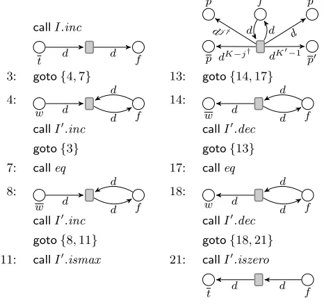
Figure 5. Performing a call`j† providedI < N −1. At the
beginning,I0is assumed to be zero, and the same is guaranteed at the end.
•The current heightiof the stack of subroutine calls is kept in one of the auxiliary counters, and we have that:
for alli0< i, the program counter of thei0th copy ofLis at some subroutine invocationcall`0such that the program counter of the(i0+ 1)th copy ofLis in the routine named`0; for alli0> i, there arehi0, N−1−i0,0,0,0,0,1itokens carryingdi0on placeshw, w, p, p, p0, p0, ti.
•For every name manipulated by the ith copy of L, hi, N − 1−i,1itokens carrying it are kept on special placeshw, w, ti. Thus, placestandtare used to distinguish these names from the artificial names that record the control.
To defineL∗, its places are all the places that occur inL, plus nine special placesw,w,p,p,p0,p0,t,tandf. WritingN for the bound of the auxiliary counters andI,I0for the two auxiliary counters, routine`j : R∗jofL
∗
is defined to execute:
•If`j =init, initialise the auxiliary counters (by calling their initroutine), and then using the auxiliary counters and place
f, for eachi∈ {0, . . . , N−1}, puthi, N−1−i,1itokens carrying a fresh namedionto placeshw, w, ti.
•Put hj, K −j,1, K0 − 1i tokens carrying d0 onto places
hp, p, p0, p0i. (Iwill always be0at this point.)
•Repeatedly, usingI0and placef, identifyj0andj00such that there are hI, N −1−I, j0, K−j0, j00, K0 −j00,1i tokens carryingdIon placeshw, w, p, p, p0, p0, ti, and advance theIth
copy ofLby performing the commandcat linej00in routine
`j0 : Rj0ofLas follows:
Ifcis aνPN transition, useI0and placefto maintain the
Ith name space, i.e. to ensure that all names manipulated by
chavehI, N−1−I,1itokens on placeshw, w, ti.
Ifcis a nondeterministic jumpgotoG, choosej‡∈Gand ensure that there arehj‡, K0−j‡itokens carryingdI on
placeshp0, p0i.
If c is a subroutine invocation call`j† and I < N −
1, put hj†, K −j†,1, K0 −1i tokens carrying dI+1 on
places hp, p, p0, p0i, and incrementI. Example code that implements this can be found in Figure 5.
Ifcis a subroutine invocationcall`0,I =N −1and`0
is not an increment or a decrement (of the trivial counter programEnum(1)), simply increment the program counter by moving a token carryingdI from placep0to placep0.
When`0is an increment or a decrement,L∗blocks at this point.
In the remaining case, c is return. Remove the tokens carryingdI from places hp, p, p0, p0i. IfI > 0, move a
token carryingdI−1 fromp0to placep0 and decrementI.
Otherwise, exit the loop.
We observe thatL∗is computable fromLin logarithmic space.
Lemma 12. For everyF-correct counter libraryL, we have that
L∗isλx.Fx(1)
-correct.
Proof.We argue by induction on N that, for every N-correct
counter programC,L∗◦CisFN(1)-correct.
The base caseN= 1is straightforward. SupposeCis1-correct, i.e. provides counters with only one possible value. By the definition ofL∗, when the bound of the auxiliary counters is1, only one copy ofL is simulated. HenceL∗◦Cas a counter program is indistinguishable fromL◦Enum(1). The latter isFN(1)-correct, i.e.F(1)-correct, becauseLis assumedF-correct andEnum(1)is 1-correct by Lemma 10.
For the inductive step, supposeCis(N+ 1)-correct. For any tape contentsM ofL∗◦Candi∈ {0, . . . , N}, letMidenote the
subcontents belonging to theith copy ofL, i.e. the restriction ofM
to the names that labelhi, N−i,1itokens on placeshw, w, tiand to the places ofL.
By the inductive hypothesis and Lemma 10,L∗◦Enum(N) is FN(1)
-correct, and so L◦(L∗ ◦Enum(N)) is FN+1(1)
-correct. For any tape contentsM0of the latter counter program andi∈ {0, . . . , N}, letMi0denote: ifi= 0, the subcontents of the
left-handL; otherwise, the subcontents belonging to the(i−1)th copy ofLinL∗◦Enum(N).
The required conclusion that L∗◦C isFN+1(1)-correct is
implied by the next claim, proven in the full paper:
Claim12.1. For every tape contentsMandM0whichL∗◦Cand
L◦(L∗◦Enum(N))(respectively) can compute from the empty tape contents by a sequenceσof counter operations whereinit occurs only as the first element, we have that:
1.Mi=Mi0for alli∈ {0, . . . , N};
2. for every counter operationop6=init,L∗◦Ccan completeop fromMif and only ifL◦(L∗◦Enum(N))can completeop fromM0.
5.5 Doubly-Ackermannian Minsky Machines
We are now equipped to reduce from the followingFω·2-complete
problem (cf. Schmitz 2016, Section 2.3.2):
Given a deterministic Minsky machineM, does it halt while the sum of counters is less thanAω·2(|M|)?
and thereby establish our lower bound. The idea here is classical: simulateMby a reset Petri net on a doubly-Ackermannian budget, and if it halts then check that the simulation was accurate.
Theorem 13. The coverability problem forνPNs isFω·2-hard.
Proof.Suppose Ma deterministic Minsky machine. Let L|M|
iteration operators. By lemmata 10, 11 and 12, we have thatL|M|
isAω+|M|+1-correct and thatL|M|◦Enum(|M|)isAω·2(|M|)
-correct. Finally, letSim(M)be a one-routine library that uses one of the pair of counters provided by the counter program
L|M|◦Enum(|M|)as follows:
•InitialiseL|M|◦Enum(|M|).
•SimulateMwhere zero tests are performed as resets (cf. Sec-tion 2.3) and where the difference between the total number of increments and the total number of decrements is maintained in a counterT ofL|M|◦Enum(|M|). Any attempt to increment
T beyond its maximum value blocks the simulation.
•IfMhalts, check that the sum of its counters is at leastT, i.e. decreaseTto zero while at each step decrementing some counter ofM.
Observe that the latter check succeeds if and only if there was no reset of a non-zero counter, i.e. all zero tests in the simulation were correct. Hence,Mhalts while the sum of its counters is less than
Aω·2(|M|)if and only if the one-routine program
Test(M) =Sim(M)◦(L|M|◦Enum(|M|))
can terminate, i.e. theνPNN(Test(M))can cover the marking in which the control places point to the last line ofTest(M).
Since the iteration operator is computable in logarithmic space and increases the number of places by adding a constant, we have that the counter libraryL|M|and thus also theνPNN(Test(M))
are computable in time elementary in|M|, and that their numbers of places are linear in|M|. We conclude theFω·2-hardness by
the closure under any sub-doubly-Ackermannian reduction (i.e. in F<ω·2), and therefore certainly any elementary one (Schmitz 2016,
Section 2.3.1).
6.
Concluding Remarks
In this paper, we have shown that coverability inν-Petri nets is complete for double Ackermann time, i.e.Fω·2-complete. In order
to solve this open problem, we have applied a new technique to analyse the complexity of the backward coverability algorithm using ideal representations—thereby demonstrating the versatility of this technique designed in (Lazi´c and Schmitz 2015)—, and pushed for the first time the ‘object oriented’ construction of Lipton (1976) beyond Ackermann-hardness. This is also the first known instance of a natural decision problem for double Ackermann time.
OurFω·2 upper bound furthermore improves the best known
upper bound for coverability in unordered data Petri nets. In this case however, the currently best known lower bound is hardness for
F3, which was proven by Lazi´c et al. already in 2008, leaving quite
a large complexity gap.
Acknowledgements
The authors thank R. Meyer and F. Rosa-Velardo for their insights into the relationships betweenπ-calculus andνPNs, and J. Goubault-Larrecq, P. Karandikar, K. Narayan Kumar, and Ph. Schnoebelen for sharing their draft paper.
References
P. A. Abdulla, K. ˇCer¯ans, B. Jonsson, and Y.-K. Tsay. Algorithmic analysis of programs with well quasi-ordered domains.Inform. and Comput., 160 (1–2):109–127, 2000.
M. Blondin, A. Finkel, and P. McKenzie. Handling infinitely branching WSTS. InProc. ICALP 2014, volume 8573 ofLNCS, pages 13–25, 2014.
R. Bonnet. On the cardinality of the set of initial intervals of a partially ordered set. InInfinite and finite sets, Vol. 1, Coll. Math. Soc. J´anos Bolyai, pages 189–198. North-Holland, 1975.
L. Bozzelli and P. Ganty. Complexity analysis of the backward coverability algorithm for VASS. InProc. RP 2011, volume 6945 ofLNCS, pages 96–109. Springer, 2011.
P. Chambart and Ph. Schnoebelen. The ordinal recursive complexity of lossy channel systems. InProc. LICS 2008, pages 205–216. IEEE Press, 2008. E. A. Cicho´n and E. Tahhan Bittar. Ordinal recursive bounds for Higman’s
Theorem.Theor. Comput. Sci., 201(1–2):63–84, 1998.
N. Decker and D. Thoma. On freeze LTL with ordered attributes. InProc. FoSSaCS 2016, volume 9634 ofLNCS, pages 269–284. Springer, 2016. D. Figueira, S. Figueira, S. Schmitz, and Ph. Schnoebelen. Ackermannian
and primitive-recursive bounds with Dickson’s Lemma. InProc. LICS 2011, pages 269–278. IEEE Press, 2011.
A. Finkel and J. Goubault-Larrecq. Forward analysis for WSTS, part I: Completions. InProc. STACS 2009, volume 3 ofLIPIcs, pages 433–444. LZI, 2009.
A. Finkel and Ph. Schnoebelen. Well-structured transition systems every-where!Theor. Comput. Sci., 256(1–2):63–92, 2001.
A. Finkel, P. McKenzie, and C. Picaronny. A well-structured framework for analysing Petri net extensions.Inform. and Comput., 195(1–2):1–29, 2004.
J. Goubault-Larrecq, P. Karandikar, K. Narayan Kumar, and Ph. Schnoebelen. The ideal approach to computing closed subsets in well-quasi-orderings. In preparation, 2016.
C. Haase, S. Schmitz, and Ph. Schnoebelen. The power of priority channel systems.Logic. Meth. in Comput. Sci., 10(4:4):1–39, 2014.
S. Haddad, S. Schmitz, and Ph. Schnoebelen. The ordinal recursive complexity of timed-arc Petri nets, data nets, and other enriched nets. In
Proc. LICS 2012, pages 355–364. IEEE Press, 2012.
G. Higman. Ordering by divisibility in abstract algebras. Proc. London Math. Soc., 3(2):326–336, 1952.
R. Lazi´c and S. Schmitz. The ideal view on Rackoff’s coverability technique. InProc. RP 2015, volume 9328 ofLNCS, pages 1–13. Springer, 2015. R. Lazi´c, T. Newcomb, J. Ouaknine, A. Roscoe, and J. Worrell. Nets with
tokens which carry data.Fund. Inform., 88(3):251–274, 2008. R. Lazi´c, J. Ouaknine, and J. Worrell. Zeno, Hercules, and the Hydra: Safety
metric temporal logic is Ackermann-complete. ACM Trans. Comput. Logic, 17(3), 2016.
R. Lipton. The reachability problem requires exponential space. Technical Report 62, Yale University, 1976.
R. Meyer. On boundedness in depth in theπ-calculus. InProc. IFIP TCS 2008, volume 273 ofIFIP AICT, pages 477–489. Springer, 2008. M. Montali and A. Rivkin. Model checking Petri nets with names using
data-centric dynamic systems.Form. Aspects Comput., 2016. To appear. C. Rackoff. The covering and boundedness problems for vector addition
systems.Theor. Comput. Sci., 6(2):223–231, 1978.
F. Rosa-Velardo. Ordinal recursive complexity of unordered data nets. Technical Report TR-4-14, Universidad Complutense de Madrid, 2014. F. Rosa-Velardo and D. de Frutos-Escrig. Name creation vs. replication in
Petri net systems.Fund. Inform., 88(3):329–356, 2008.
F. Rosa-Velardo and D. de Frutos-Escrig. Decidability and complexity of Petri nets with unordered data.Theor. Comput. Sci., 412(34):4439–4451, 2011.
F. Rosa-Velardo and M. Martos-Salgado. Multiset rewriting for the veri-fication of depth-bounded processes with name binding. Inform. and Comput., 215:68–87, 2012.
S. Schmitz. Complexity hierarchies beyond Elementary. ACM Trans. Comput. Theory, 8(1):1–36, 2016.
S. Schmitz and Ph. Schnoebelen. Multiply-recursive upper bounds with Higman’s Lemma. InProc. ICALP 2011, volume 6756 ofLNCS, pages 441–452. Springer, 2011.
S. Schmitz and Ph. Schnoebelen. Algorithmic aspects of WQO theory. Lecture notes, 2012. URLhttp://cel.archives-ouvertes.fr/ cel-00727025.
S. Schmitz and Ph. Schnoebelen. The power of well-structured systems. In
Proc. Concur 2013, volume 8052 ofLNCS, pages 5–24. Springer, 2013. Ph. Schnoebelen. Revisiting Ackermann-hardness for lossy counter
ma-chines and reset Petri nets. InProc. MFCS 2010, volume 6281 ofLNCS, pages 616–628. Springer, 2010.