Mathematical Background: Consider a simple discrete-time transfer function with input R z and

1

ECE-420: Discrete-Time Control Systems

Project Part A: Simulating a Plant

In this part of the project you will simulate a few discrete-time systems in both Matlab and Simulink to see how the embedded systems toolbox works. You will need to download the project files from the class website for this. The embedded system toolbox may not work with 64 bit systems.

Mathematical Background: Consider a simple discrete-time transfer function with input R z( ) and output Y z( ),

1 2

0 1 2

1 2

1 2

( ) ( )

( ) (

( ) )

1

b b z b z

Y z B z

R z a

G

z a z A z

z

− −

− −

+ +

= =

=

+ +

Cross multiplying we get

1 2 1 2

1 ( ) 2 0 1 2

( )z z Y z z Y z( ) b R z( ) b z R z( ) b z ( )z

Y +a − +a − = + − + − R

In the time-domain this becomes

1 2 0 1 2

( ) ( 1) ( 2) ( ) ( 1) ( 2)

y n = −a y n− −a y n− +b r n +b r n− +b r n−

In Matlab, theAandBarrays are then

[

]

[

]

1 2

0 1 2

1

A a a

B b b b

= =

In Matlab, there will be an equal number of elements in both arrays and they are row arrays (because of the way we constructed them). Let’s assume that N denotes the maximum number of coefficients in the transfer function. Then to implement this algorithm to find the current output y n( )we need the current input r n( ) and the previous N-1 inputs and outputs. This fact is important to understand what is going on in the tapped delays in the Simulink model.

We can then determine the current output using the following Matlab loop

y(n) = B(1)*r(n) for k=2:N

y(n) = y(n) - A(k)*y(n-k+1) + B(k)*r(n-k+1) end;

2 1) Open the files openloop_DE.mdl and openloop_driver.m. These files generate both a Matlab and a Simulink simulation of the unit step response for the discrete-time transfer function

1

1 1

0. ( )

1 0.8 8

p

z z G

z z

− −

= =

− −

In this case we have A=

[

]

[

]

Run openloop_driver.m, you should get the graph shown in Figure 1, however, it may take awhile. This figure shows the results from the Matlab and Simulink simulations are identical, which is a good way to check your answers.

. Figure 1. Open loop response of the system.

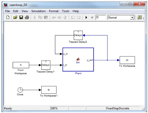
2) Now open up openloop_DE.mdl (double click on it). It should look like Figure 2. We will be going through a number of the elements in this model.

Figure 2. openloop_DE.mdl

0 0.5 1 1.5 2 2.5 3

0 0.5 1 1.5 2 2.5 3 3.5 4 4.5 5

Time

y

v

al

ue

3 Before we get too far, there is a sort of logic to some of the parameter names used in this model. First of all, Ap and Bp refer to the A and B vectors of coefficients for the plant transfer function. This is to (later) differentiate them from Ac and Bc, which will be vectors of coefficients for the controller

transfer function. Similarly, the parameter Nbp indicates the number of elements in the Bp array (and by default, the Ap array). Later we will use Nbc to indicate the number of elements in the Bc and Ac

arrays. The variable r_in is the input to the plant, the variable y_out is the output of the plant, and the variable y_in is the output fed back to the input (with delays).

Starting at the left of the model (Figure 2), the input goes into a Delay Block. If you click on the delay block you will get the parameter block shown in Figure 3. This figure also shows what many of the parameters mean.

Figure 3. Parameter block for first delay, with explanations.

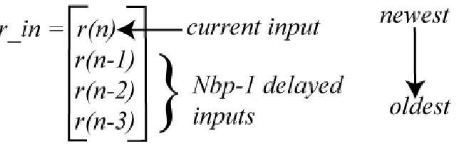
For Nbp = 4, the output of this delay block looks like the vector depicted in Figure 4. Note that Matlab uses a column vector of values for the output of a Delay block. This is important to remember!

Figure 4. Output of the first Delay block, for Nbp = 4. The data is sorted from newest to oldest, the data includes the current input, and there are Nbp-1=3 delays. Note that Matlab uses a column vector of values for the output of a Delay block.

Initial Conditions are 0 _{Inherit the sample time}

We need Nbp-1 delayed values, plus the current value

Order the output with the newest element first

4 If we look at the Delay block used in feeding the output back into the system (at the top of Figure 2), it looks like that shown in Figure 5. This is very similar to the Delay block shown in Figure 3. The only difference is the current input is not included in the output. The output of this block for Nbp = 4 is shown in Figure 6.

Figure 5. Delay block used for feeding the output back into the system.

Figure 6. Output of the delay block feeding the output back into the system for Nbp = 4. Note that Matlab uses a column vector of values for the output of a Delay block.

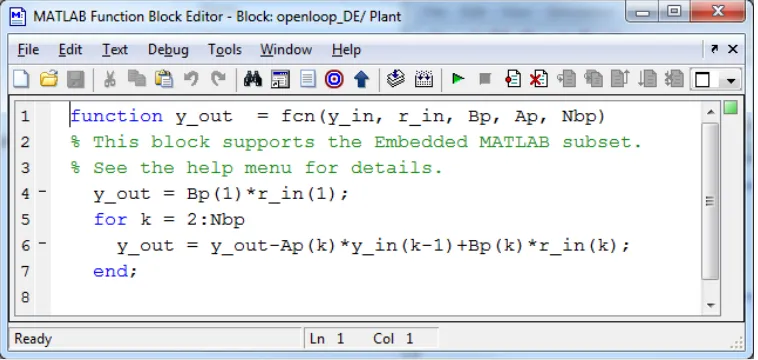
Now click on the plant (the large block in the center of Figure 2) and you will get the innocent looking piece of code for implementing a discrete-time transfer function shown in Figure 7. There are five things “passed” to this function: y_in, r_in, Bp, Ap, and Nbp.

Figure 7. Code inside the plant block for implementing a discrete-time transfer function. Note the current input is

5 Click on the Edit Data/Ports icon, as shown in Figure 8, to access the variables.

Figure 8. Accessing the “passed” items to this block via the Edit Data/Ports icon.

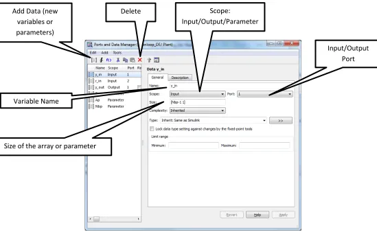
Once you click on the Edit Data/Ports icon, you will get a window like that shown in Figure 9.

Figure 9. Modifying variables and parameters. There are many things that can be varied. The ones you are most likely to change have been highlighted.

Delete

Variable Name

Input/Output Port Scope:

Input/Output/Parameter

Size of the array or parameter Add Data (new

6 Referring to Figure 9,

• If the scope is a parameter, then you should not expect it to change as the simulation is running. Thus, Nbp, Bp, and Ap are parameters. If the scope is an input or output, then you should expect it to change as the simulation is running, such as y_in, r_in, and y_out.

• The port indicates the order in which the variable will appear in the left (input) or right (output) side of the block. For this simulation, the port of y_in is one and the port of r_in is two, and this is reflected in how they are placed on the left of the plant block (See Figure 2).

• Most likely you will be changing the Size of the variables more than anything else. It is a good idea (for the problems you are likely to get) to try and not hard-code numbers and use parameters like Nbp, Nbp-1, etc. Note that for this example, Bp and Ap are row vectors with size [1 Nbp], while y_in and r_in are column vectors, with sizes [Nbp-1 1] and [Nbp 1], respectively.

• Add Data allows you to add new variables and parameters.

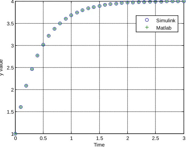
3) Modify the code as needed to determine the step response of the discrete-time plant

1

1 1 0.2 ( )

1 0.8

p

z z

z G

− −

− =

−

Assume a sampling interval of 0.1 seconds and run the simulation for 3 seconds. You should get a plot like that shown in Figure 10. Include your plot in your memo

Figure 10. Step response for

1

1 1 0.2 ( )

1 0.8

p

z z

z G

− −

− =

−

0 0.5 1 1.5 2 2.5 3

1 1.5 2 2.5 3 3.5 4

Time

y

v

al

ue

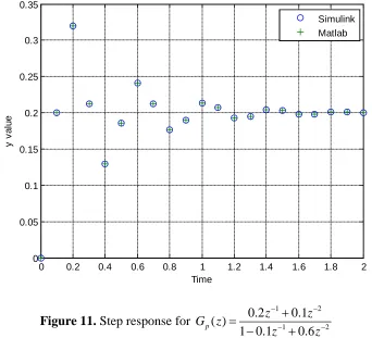
7 4) Modify the code as needed to determine the step response of the discrete-time plant

1 2 1 2 0 0.2 ( ) 1 0. .1 0 6 1 . p z G z z z z − − − ₊ − − + =

Assume a sampling interval of 0.1 seconds and run the simulation for 2 seconds. You should get a plot like that shown in Figure 11. Include your plot in your memo.

Figure 11. Step response for

1 2 1 2 0 0.2 ( ) 1 0. .1 0 6 1 . p z G z z z z − − − ₊ − − + =

To turn in: write a short memo including your graphs (with captions and figure numbers), and any suggestions you may have for improving this part of the project. E-mail me your memo.

0 0.2 0.4 0.6 0.8 1 1.2 1.4 1.6 1.8 2