Portfolio Optimization with Reward-Risk Ratio
Measure based on the Conditional Value-at-Risk
Wlodzimierz Ogryczak, Michał Przyłuski, Tomasz ´Sliwi´nski
Abstract—In several problems of portfolio selection the reward-risk ratio criterion is optimized to search for a risky portfolio offering the maximum increase of the mean return, compared to the risk-free investment opportunities. We analyze such a model with the CVaR type risk measure. Exactly the deviation type of risk measure must be used, i.e. the so-called conditional drawdown measure. We analyze both the theoretical properties (SSD consistency) and the computational complexity (LP models).
Index Terms—portfolio optimization, reward-risk ratio, conditional-value-at-risk, linear programming, stochastic dom-inance.
I. INTRODUCTION
P
ORTFOLIO selection problems are usually tackled with the mean-risk models that characterize the uncertain returns by two scalar characteristics: the mean, which is the expected return, and the risk - a scalar measure of the variability of returns. In the original Markowitz model the risk is measured by the standard deviation or variance. Several other risk measures have been later considered thus creating the entire family of mean-risk (Markowitz-type) models. While the original Markowitz model forms a quadratic programming problem [1], many attempts have been made to linearize the portfolio optimization procedure (c.f., [2], [3] and references therein). The LP solvability is very important for applications to real-life financial decisions where the constructed portfolios have to meet numerous side constraints (including the minimum transaction lots, trans-action costs and mutual funds characteristics). In order to guarantee that the portfolio takes advantage of diversification, no risk measure can be a linear function of the portfolio weights. Nevertheless, a risk measure can be LP computable in the case of discrete random variables, i.e., in the case of returns defined by their realizations under specified scenarios. The simplest LP computable risk measures are disper-sion measures similar to the variance. The mean absolute deviation was very early considered in portfolio analysis [4] while [5] presented and analyzed the complete portfolio optimization model (the so-called MAD model). Yitzhaki [6] introduced the mean-risk model using Gini’s mean (absolute) difference as the risk measure. Both the mean absolute de-viation and the Gini’s mean difference turn out to be special aggregation techniques of the multiple criteria LP model [7] based on the pointwise comparison of the absolute Lorenz curves. The latter leads the quantile shortfall risk measures which are more commonly used and accepted. Recently, theManuscript received July 8, 2015; revised July 28, 2015. This work was supported in part by the National Science Centre (Poland) under the grant DEC-2012/07/B/HS4/03076.
W. Ogryczak, M. Przyłuski and T. ´Sliwi´nski are with the Institute of Control and Computation Engineering, Warsaw University of Technology, Poland, e-mail:{w.ogryczak, m.przyluski, t.sliwinski}@elka.pw.edu.pl.
second order quantile risk measures have been introduced in different ways by many authors [8], [9], [10]. The measure, now commonly called the Conditional Value at Risk (CVaR) (after [10] or Tail VaR, represents the mean shortfall at a specified confidence level. It leads to LP solvable portfolio optimization models in the case of discrete random variables represented by their realizations under specified scenarios. The CVaR has been shown by [11] to satisfy the requirements of the so-called coherent risk measures [8] and is consistent with the second degree stochastic dominance as shown by [12]. Several empirical analyses [13], [14], [15] confirm its applicability to various financial optimization problems.
In this paper we analyze the reward-risk ratio criterion is optimized to search for a risky portfolio offering the maximum increase of the mean return, compared to the risk-free investment opportunities. We analyze such a model with the CVaR type risk measure. Exactly the deviation type of risk measure must be used, i.e. the so-called conditional drawdown measure. Both the theoretical properties and the computational complexity are analyzed. In Section III we show that under natural restriction on the target value the CVaR reward-risk ratio optimization is SSD consistent. Fur-ther in Section IV we show that while carefully transforming the CVaR risk-reward ratio optimization to an LP model and taking advantages of the LP duality we are able to get a model formulation providing high computational efficiency.
II. PORTFOLIO OPTIMIZATION ANDCVARMEASURES
W
E consider a situation where an investor intends tooptimally select a portfolio of assets and hold it until the end of a defined investment horizon. Let J = {1,2, . . . , n} denote a set of assets available for the invest-ment. For each assetj∈J, its rate of return is represented by a random variable (r.v.)Rj with a given meanµj=E{Rj}. Furthermore, letx= (xj)j=1,...,ndenote a vector of decision variablesxj representing the shares (weights) that define a portfolio of assets. To represent a portfolio, these weights must satisfy a set of constraints. The basic set of constraints includes the requirement that the weights must sum to one, i.e., Pn
j=1xj = 1, and that short sales are not allowed, i.e., xj ≥ 0 for j = 1, . . . , n. An investor usually needs to consider some other requirements expressed as a set of additional side constraints. Most of them can be expressed as linear equations and inequalities. We will assume that the basic set of feasible portfoliosQ, i.e. the set of solutions that do not violate the basic set of constraints mentioned above, is a general LP feasible set given in a canonical form as a system of linear equations with nonnegative variables.
Each portfolio x defines a corresponding r.v. Rx = Pn
E{Rx} = P n
j=1µjxj. We consider T scenarios, each one with probability pt, where t = 1, . . . , T. We assume that, for each r.v.Rj, its realizationrjtunder scenariotis known and that, for each asset j, j = 1, . . . , n, its mean rate of return is computed as µj =PTt=1rjtpt. The realization of the portfolio rate of return Rx under scenariot is given by yt=P
n
j=1rjtxj.
The portfolio optimization problem considered in this pa-per follows the original Markowitz’ formulation and is based on a single period model of investment. At the beginning of a period, an investor allocates the capital among various assets, thus assigning a nonnegative weight (share of the capital) to each asset. Let J = {1,2, . . . , n} denote a set of assets considered for an investment. For each asset j∈J, its rate of return is represented by a random variable Rj with a given mean µj = E{Rj}. Further, let x = (xj)j=1,2,...,n denote a vector of decision variables xj expressing the weights defining a portfolio. The weights must satisfy a set of constraints to represent a portfolio. The simplest way of defining a feasible setQis by a requirement that the weights must sum to one and they are nonnegative (short sales are not allowed), i.e.
Q={x :
n
X
j=1
xj= 1, xj ≥0 for j= 1, . . . , n} (1)
Hereafter, we perform detailed analysis for the set Qgiven with constraints (1). Nevertheless, the presented results can easily be adapted to a general LP feasible set given as a system of linear equations and inequalities.
Each portfolioxdefines a corresponding random variable Rx = Pn
j=1Rjxj that represents the portfolio rate of
return while the expected value can be computed asµ(x) = Pn
j=1µjxj. We consider T scenarios with probabilities pt (where t = 1, . . . , T). We assume that for each random variableRj its realizationrjtunder the scenariotis known. Typically, the realizations are derived from historical data treating T historical periods as equally probable scenarios (pt = 1/T). Although the models we analyze do not take advantages of this simplification. The realizations of the portfolio return Rx are given asyt=P
n
j=1rjtxj.
The portfolio optimization problem is modeled as a mean-risk bicriteria optimization problem where the meanµ(x)is maximized and the risk measure %(x) is minimized. In the original Markowitz model, the standard deviation was used as the risk measure. Several other risk measures have been later considered thus creating the entire family of mean-risk models (c.f., [15], [16]). These risk measures, similar to the standard deviation, are law-invariant (are not affected by any shift of the outcome scale) and are risk relevant (equal to 0 in the case of a risk-free portfolio while taking positive values for any risky portfolio). Unfortunately, such risk measures are not consistent with the stochastic dominance order [17] or other axiomatic models of risk-averse preferences [18] and coherent risk measurement [8].
In stochastic dominance, uncertain returns (modeled as random variables) are compared by pointwise comparison of some performance functions constructed from their dis-tribution functions. The first performance function Fx(1) is defined as the right-continuous cumulative distribution func-tion: Fx(1)(η) = Fx(η) = P{Rx ≤ η} and it defines the
first degree stochastic dominance (FSD). The second function is derived from the first as Fx(2)(η) = R
η
−∞Fx(ξ) dξ and it defines the second degree stochastic dominance (SSD). We say that portfolio x0 dominates x00 under the SSD (Rx0
SSD Rx00), ifF
(2)
x0 (η)≤F
(2)
x00(η)for allη, with at least one strict inequality. A feasible portfolio x0 ∈ Q is called SSD efficient if there is nox∈Q such thatRxSSD Rx0.
Stochastic dominance relates the notion of risk to a possible failure of achieving some targets. As shown by [19], function Fx(2), used to define the SSD relation, can also be presented as follows:Fx(2)(η) =E{max{η−Rx,0}}and thereby its values are LP computable for returns represented by their realizationsyt.
An alternative characterization of the SSD relation can be achieved with the so-called Absolute Lorenz Curves (ALC) [9] which represent the second quantile functions defined as Fx(−2)(0) = 0and
Fx(−2)(p) = Z p
0
Fx(−1)(α)dα for0< p≤1, (2)
where Fx(−1)(p) = inf {η : Fx(η) ≥ p} is the left-continuous inverse of the cumulative distribution function Fx. The pointwise comparison of ALCs is equivalent to the SSD relation [12] in the sense that Rx0 SSD Rx00 if and only ifFx(−0 2)(β)≥F
(−2)
x00 (β)for all0< β ≤1. Moreover,
Fx(−2)(β) = max η∈R
h
βη−Fx(2)(η)i
= max
η∈R [βη−E{max{η−Rx,0}}] (3)
where η is a real variable taking the value of β-quantile Qβ(x)at the optimum. For a discrete r.v. represented by its realizationsyt problem (3) becomes an LP.
For any real tolerance level 0 < β ≤ 1, the normalized value of the ALC defined as
Mβ(x) =Fx(−2)(β)/β (4)
is called theConditional Value-at-Risk (CVaR)or Tail VaR or Average VaR. The CVaR measure is an increasing function of the tolerance level β, with M1(x) = µ(x). For any 0 < β <1, the CVaR measure is SSD consistent [12] and coherent [11]. Opposite to deviation type risk measures, for coherent measures larger values are preferred and therefore the measures are sometimes called safety measures [15]. Due to (3), for a discrete random variable represented by its realizationsyt the CVaR measures are LP computable. It is important to notice that although the quantile risk measures (VaR and CVaR) were introduced in banking as extreme risk measures for very small tolerance levels (likeβ= 0.05), for the portfolio optimization good results have been provided by rather larger tolerance levels [15].
For β approaching 0, the CVaR measure tends to the Minimax measure
M(x) = min
t=1,...,Tyt (5) introduced to portfolio optimization by Young [20]. Note that the maximum (downside) semideviation
∆(x) =µ(x)−M(x) = max
t=1,...,T(µ(x)−yt) (6) and the conditionalβ-deviation
respectively, represent the corresponding deviation risk mea-sures. They may be interpreted as the drawdown measures [21]. For β= 0.5the measure ∆0.5(x)represents the mean
absolute deviation from the median [16].
The commonly accepted approach to implementation of the Markowitz-type mean-risk model (with deviation type risk measures) is based on the use of a specified lower bound µ0 on expected returns while optimizing the risk measure.
This bounding approach provides a clear understanding of investor preferences and a clear definition of optimal port-folio to be sought. For deviation type risk measures % the approach results in the following minimum risk problem:
min{%(x) : µ(x)≥µ0, x∈Q} (8)
While using the coherent and SSD consistent risk measures µ% one may focus on the measure maximization without additional constraints
max{µ%(x) : x∈Q} (9)
or still consider some preferential constraints on the mean expectation
max{µ%(x) : µ(x)≥µ0, x∈Q}. (10)
In the case of CVaR measure both models can be effectively solved for large numbers of scenarios while taking advan-tages of appropriate dual formulations [22].
III. REWARD-RISK RATIO OPTIMIZATION
A
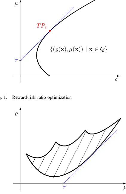
N alternative specific approach to portfolio optimization looks for a risky portfolio offering the maximum in-crease of the mean return, compared to the risk-free targetτ. Namely, given the risk-free rate of returnτ, a risky portfoliox that maximizes the ratio(µ(x)−τ)/%(x)is sought. This leads us to the following ratio optimization problem:
max µ(x)
−τ
%(x) : x∈Q
. (11)
The approach is well appealing with respect to the prefer-ences modeling and applied to standard portfolio selection or (extended) index tracking problems (with a benchmark as the target). We illustrate ratio optimization (11) in Fig. 1. For the LP computable risk measures the reward-risk ratio optimization problem can be converted into an LP form [16]. When the risk-free returnr0is used instead of the targetτ
than the ratio optimization (11) corresponds to the classical Tobin’s model [23] of the modern portfolio theory (MPT) where the capital market line (CML) is the line is drawn from the risk-free rate at the intercept that passes tangent to the mean-risk efficient frontier. Any point on this line provides the maximum return for each level of risk. The tangency (tangent, super-efficient) portfolio is the portfolio of risky assets on the efficient frontier at the point where the CML is tangent to the efficiency frontier. It is a risky portfolio offering the maximum increase of the mean return while comparing to the risk-free investment opportunities. Namely having given the risk-free rate of returnr0 one seeks a risky
portfolio xthat maximizes the ratio(µ(x)−r0)/%(x).
Instead of the reward-risk ratio maximization one may consider an equivalent model of the risk-reward ratio mini-mization (see Fig. 2):
min
%(x)
µ(x)−τ : x∈Q
. (12)
6
-µ
%
{(%(x), µ(x))|x∈Q}
τ
r
[image:3.595.313.524.55.379.2]T Pτ
Fig. 1. Reward-risk ratio optimization
6
-%
µ
[image:3.595.307.548.626.735.2]
τ
Fig. 2. Risk-reward ratio optimization
Actually, this is a classical model for the tangency portfolio as considered by Markowitz [1] and used in statistics books [24].
Both the ratio optimization models (11) and (12) are theo-retically equivalent. However the risk-reward ratio optimiza-tion (12) enables easy control of the denominator positivity by simple inequality µ(x)≥τ+ε added to the problem constraints. The model may also be additionally regularized for the case of multiple risk-free solutions. Regularization
(%(x) +ε)/(µ(x)−τ)guarantees that the risk-free portfolio with the highest mean return will be selected then.
Theorem 1: If risk measure%(x)is mean-complementary SSD consistent, i.e.
Rx0
SSD Rx00 ⇒ µ(x
0)−%(x0)≥µ(x00)−%(x00)
then the reward-risk ratio optimization (11) or equivalently (12) is SSD consistent provided that µ(x) > τ > µ(x)−
%(x).
Proof:Note that
−1 + %(x)
µ(x)−τ =
τ−(µ(x)−%(x))
µ(x)−τ .
IfRx0
SSDRx00, thenµ(x
0)−%(x0)≥µ(x00)−%(x00)and
µ(x0)≥µ(x00). Hence,
τ−(µ(x0)−%(x0))
µ(x0)−τ ≥
τ−(µ(x00)−%(x00))
µ(x00)−τ
provided that both numerators and denominators remains positive.
model we must replace this performance measure (coherent risk measure) with its complementary deviation represen-tation. The deviation type risk measure complementary to theCV aRβ representing the tail mean within theβ-quantile takes the form of ∆β(x) =µ(x)−CV aRβ(x)(conditional semideviation or drawdown measure) thus leading to the ratio optimization [16]:
µ(x)−τ
∆β(x)
→ max (13)
Taking advantages of possible inverse formulation of the risk-reward ratio optimization (12) as ratio
∆β(x)
µ(x)−τ → min (14)
we get a model well defined for µ(x) > τ and SSD consistent for τ − Mβ(x) ≥ 0. Thus, this CVaR ratio optimization is consistent with the SSD rules (similar to the standard CVaR optimization [12]), despite that the ratio does not represent a coherent risk measure [8].
Theorem 2: For any target level τ such that there exists portfolio x ∈ Q satisfying requirements τ ≥ Mβ(x) and µ(x)−τ≥ε >0, except for portfolios with identical values of the corresponding CVaR risk-reward ratio, every optimal solution of the problem
min
∆β(x)
µ(x)−τ :x∈Q, τ ≥Mβ(x), µ(x)−τ ≥ε
(15)
is an SSD efficient portfolio.
Proof: Let x0 be an optimal portfolio for ratio
opti-mization (15). If there exists portfolio x ∈ Q satisfying requirements τ ≥ Mβ(x) and µ(x)−τ ≥ ε such that RxSSD Rx0, then following Theorem 1
∆β(x) µ(x)−τ ≤
∆β(x0) µ(x0)−τ.
Hence, due to optimality ofx0
∆β(x) µ(x)−τ =
∆β(x0) µ(x0)−τ.
which completes the proof.
IV. COMPUTATIONALLP MODELS
I
N this section we will show that while transforming the CVaR risk-reward ratio optimization (14) to an LP model, we can take advantages of the LP duality to get a model formulation providing higher computational efficiency. In the introduced model, similar to the direct CVaR optimization [25], the number of structural constraints is proportional to the number of instruments while only the number of variables is proportional to the number of scenarios, thus not affecting so seriously the simplex method efficiency. The model can effectively be solved with general LP solvers even for very large numbers of scenarios (like the case of fifty thousand scenarios and one hundred instruments solved less than a minute). On the other hand such efficiency cannot be achieved with model (13).Let us consider portfolio optimization problem with asset returns given by discrete random variables with realization rjt thus leading to LP models for coherent risk measures we consider. Let us focus first on measures maximization
without additional (preferential) constraints thus considering the optimization models of type (9).
Following (3) and (4), the CVaR portfolio optimization model can be formulated as the following LP problem:
max y−1
β T
X
t=1
ptdt
s.t. n
X
j=1
xj = 1, xj ≥0 j= 1, . . . , n
dt≥y− n
X
j=1
rjtxj, dt≥0 t= 1, . . . , T (16)
wherey is unbounded variable. Except from the core port-folio constraints (1), model (16) contains T nonnegative variables dt plus single η variable and T corresponding linear inequalities. Hence, its dimensionality is proportional to the number of scenariosT. Exactly, the LP model contains T+n+ 1variables andT+ 1constraints. It does not cause any computational difficulties for a few hundreds scenarios as in several computational analysis based on historical data [26]. However, in the case of more advanced simulation models employed for scenario generation one may get several thousands scenarios. This may lead to the LP model (16) with huge number of variables and constraints thus decreasing the computational efficiency of the model. As shown in [25], the computational efficiency can easily be achieved by taking advantages of the LP dual to model (16). The LP dual model takes the form:
min q
s.t. q−
T
X
t=1
rjtut≥0 j= 1, . . . , n
T
X
t=1
ut= 1
0≤ut≤ pt
β t= 1, . . . , T
(17)
containingT variablesut, but theT constraints correspond-ing to variablesdtfrom (16) take the form of simple upper bounds (SUB) onutthus not affecting the problem complex-ity. Actually, the number of constraints in (17) is proportional to the total of portfolio size n, thus it is independent from the number of scenarios. Exactly, there areT + 1variables andn+ 1constraints. This guarantees a high computational efficiency of the dual model even for very large number of scenarios.
For an LP computable risk measure %(x), the ratio optimization problem (11) can be converted into an LP form by the following transformation: introduce variables v =µ(x)/%(x) andv0 = 1/%(x), then replace the original
decision variablesxj withx˜j =xj/%(x), getting the linear criterion max v −τ v0 and an LP feasible set. Once the
transformed problem is solved the values of the portfolio variables xj can be found by dividing x˜j by v0 while
%(x) = 1/v0 andµ(x) =v/v0.
In the CVaR model, risk measure %(x) = ∆β(x) is not directly represented. We can introduce, however, the equation:
z−y+ 1
β T
X
t=1
allowing us to represent∆β(x)with variablez0. Hence, the
ratio model takes the form:
max z−τ
z0
s.t.
z−y+ 1
β T
X
t=1
ptdt=z0
dt+yt≥y, dt≥0 t= 1, . . . , T n
X
j=1
µjxj=z
n
X
j=1
rjtxj =yt t= 1, . . . , T
n
X
j=1
xj= 1, xj≥0 j = 1, . . . , n
(18)
Introducing variables v = z/z0 and v0 = 1/z0 we get
linear criterion v −τ v0 of the corresponding ratio model.
Further, we divide all the constraints by z0 and make the
substitutions: d˜t =dt/z0, y˜t =yt/z0 for t = 1, . . . , T, as
well asx˜j=xj/z0, forj= 1, . . . , nandy˜=y/z0. Finally,
we get the following LP formulation:
max v−τ v0
s.t.
v−y˜+ 1
β T
X
t=1
ptd˜t= 1
˜
dt+ ˜yt≥y,˜ d˜t≥0 t= 1, . . . , T n
X
j=1
µjx˜j=v
n
X
j=1
rjtx˜j= ˜yt t= 1, . . . , T
n
X
j=1 ˜
xj =v0, x˜j≥0 j= 1, . . . , n
(19)
After eliminating defined by equations variables v, v0 and
yt, one gets the most compact formulation:
max
n
X
j=1
µjx˜j−τ n
X
j=1 ˜
xj
s.t. −˜y+
n
X
j=1
µj˜xj+
1
β T
X
t=1
ptd˜t= 1
˜
y−
n
X
j=1
rjtx˜j−d˜t≤0 t= 1, . . . , T
˜
dt≥0 t= 1, . . . , T
˜
xj≥0 j= 1, . . . , n
(20)
that containsT+n+ 1variables andT+ 1constraints. Even taking advantages of the LP dual formulation
min q
s.t. −q+
T
X
t=1
ut= 0
µjq− T
X
t=1
rjtut≥µj−τ j= 1, . . . , n
pt
βq−ut≥0 t= 1, . . . , T ut≥0 t= 1, . . . , T
(21)
one cannot get any model that contains less thanT+n+ 1
constraints andT+ 1variables.
The complexity can be reduced however while using the risk-reward ratio optimization (12). The corresponding CVaR model takes the following form:
min
z−y+ 1
β T
X
t=1
ptdt
z−τ
s.t. dt≥y− n
X
j=1
rjtxj, dt≥0 t= 1, . . . , T
z=
n
X
j=1
µjxj, n
X
j=1
xj = 1
xj≥0, j= 1, . . . , n
(22)
It can be linearized by substitutions: d˜t = dt/(z−τ),
˜
y = y/(z−τ), x˜j = xj/(z−τ), v = z/(z−τ) and v0= 1/(z−τ) leading to the following LP formulation:
min v−y˜+ 1
β T
X
t=1
ptd˜t
s.t. d˜t≥y˜− n
X
j=1
rjtx˜j, d˜t≥0 t= 1, . . . , T
v−v0τ = 1
v=
n
X
j=1
µjx˜j, n
X
j=1 ˜
xj=v0
˜
xj≥0 j = 1, . . . , n
(23)
After eliminating defined by equations variables v and v0,
one gets the most compact formulation:
min
n
X
j=1
µjx˜j−y˜+
1
β T
X
t=1
ptd˜t
s.t. d˜t≥y˜− n
X
j=1
rjtx˜j, d˜t≥0 t= 1, . . . , T
n
X
j=1
(µj−τ)˜xj = 1, x˜j ≥0 j= 1, . . . , n (24)
The original values ofxj can be then recovered dividing ˜xj byv0.
Taking the LP dual to model (24) ones get the model:
max q
s.t. T
X
t=1
ut= 1
T
X
t=1
rjtut+ (µj−τ)q≤µj j = 1, . . . , n
0≤ut≤ pt
β t= 1, . . . , T
(25)
Similarly to experiments with CVaR computational models efficiency [25], we have run computational tests on large scale instances developed by Lim et al. [27]. They were originally generated from a multivariate normal distribution for 50, 100 or 200 assets with the number of scenarios 50,000. All computations were performed on a PC with the Intel Core i7 2.66GHz processor and 6GB RAM employing the simplex code of the CPLEX 12.5 package. An attempt to solve the CVaR reward-risk ratio model in its primal (20) or dual (21) forms with β = 0.05 resulted in similar high computations times of 620, 1487, 5102 seconds and of 656, 1544,5347 seconds on average, for problems with 50, 100 and 200 assets, respectively. For the CVaR risk-reward ratio model in its primal form (24) the computation time were remarkably higher than those for the reward-risk ratio, resulting in 864, 1749,5273 seconds on average. On the other hand, solving the dual models (25) directly by the primal method (standard CPLEX settings) resulted in dramatically shorter computation times 5.8, 14.2 and 39.9
CPU seconds, respectively. Thus, similar to the standard CVaR optimization [25], the dual model for the CVaR risk-reward ratio optimization allows one to solve effectively large scale problems. Moreover, the computation times remain very low for various tolerance levelsβ as shown in Table I.
TABLE I
COMPUTATIONAL TIMES(IN SECONDS)FOR THE DUALLPMODEL(25) OF THECVARRISK-REWARD RATIO OPTIMIZATION(AVERAGES OF10
INSTANCES WITH50,000SCENARIOS)
n β= 0.05 β= 0.1 β= 0.2 β= 0.3 β= 0.4 50 5.8 7.5 9.2 9.5 10.9
100 14.2 18.3 23.1 24.2 26.1
200 39.9 53.1 66.8 76.1 77.3
V. CONCLUSION
W
E have presented the reward-risk ratio optimization model for the CVaR risk measure and analyzed its properties. Taking advantages of possible inverse formulation of the risk-reward ratio optimization (14) we get a model well defined and SSD consistent under natural restriction on the target value selection. Thus, this CVaR ratio optimization is consistent with the SSD rules (similar to the standard CVaR optimization [12]), despite that the ratio does not represent a coherent risk measure [8].We show that while transforming the CVaR risk-reward ratio optimization (14) to an LP model, we can take ad-vantages of the LP duality to get a model formulation providing higher computational efficiency. In the introduced dual model, similar to the direct CVaR optimization [25], the number of structural constraints is proportional to the number of assets while only the number of variables is proportional to the number of scenarios, thus not affecting so seriously the simplex method efficiency. The model can effectively be solved with general LP solvers even for very large numbers of scenarios. Actually, the dual CVaR ratio portfolio optimization problems of fifty thousand scenarios and two hundred instruments can be solved with the general purpose LP solvers in less than a minute. On the other hand, such efficiency cannot be achieved with model the standard CVaR reward-risk ratio model (13).
REFERENCES
[1] H. M. Markowitz, Portfolio Selection: Efficient Diversification of Investments. New York: John Wiley & Sons, 1959.
[2] R. Mansini, W. Ogryczak, and M. G. Speranza, “Twenty years of linear programming based portfolio optimization,”European Journal of Operational Research, vol. 234, no. 2, pp. 518–535, 2014. [3] ——,Linear and Mixed Integer Programming for portfolio
optimiza-tion. Springer International Publishing, 2015.
[4] W. F. Sharpe, “Mean-absolute deviation characteristic lines for securi-ties and portfolios,”Management Science, vol. 18, pp. B1–B13, 1971. [5] H. Konno and H. Yamazaki, “Mean–absolute deviation portfolio optimization model and its application to tokyo stock market,” Man-agement Science, vol. 37, pp. 519–531, 1991.
[6] S. Yitzhaki, “Stochastic dominance, mean variance, and Gini’s mean difference,”American Economic Revue, vol. 72, pp. 178–185, 1982. [7] W. Ogryczak, “Multiple criteria linear programming model for
port-folio selection,”Annals of Operations Research, vol. 97, no. 1-4, pp. 143–162, 2000.
[8] P. Artzner, F. Delbaen, J.-M. Eber, and D. Heath, “Coherent measures of risk,”Mathematical Finance, vol. 9, no. 3, pp. 203–228, 1999. [9] W. Ogryczak, “Stochastic dominance relation and linear risk
mea-sures,” in Financial Modelling–Proc. 23rd Meeting EURO WG Fi-nancial Modelling, Cracow, 1998, A. M. Skulimowski, Ed. Progress & Business Publisher, 1999, pp. 191–212.
[10] R. T. Rockafellar and S. Uryasev, “Optimization of conditional value-at-risk,”Journal of Risk, vol. 2, pp. 21–41, 2000.
[11] G. C. Pflug, “Some remarks on the value-at-risk and the conditional value-at-risk,” in Probabilistic Constrained Optimization: Methodol-ogy and Applications, S. Uryasev, Ed. Boston: Kluwer, 2000, pp. 272–281.
[12] W. Ogryczak and A. Ruszczy´nski, “Dual stochastic dominance and related mean-risk models,” SIAM Journal on Optimization, vol. 13, no. 1, pp. 60–78, 2002.
[13] F. Andersson, H. Mausser, D. Rosen, and S. Uryasev, “Credit risk optimization with conditional value-at-risk criterion,” Mathematical Programming, vol. 89, no. 2, pp. 273–291, 2001.
[14] R. Rockafellar and S. Uryasev, “Conditional value-at-risk for general loss distributions,”Journal of Banking & Finance, vol. 26, no. 7, pp. 1443–1471, 2002.
[15] R. Mansini, W. Ogryczak, and M. G. Speranza, “LP solvable models for portfolio optimization: A classification and computational compari-son,”IMA Journal of Management Mathematics, vol. 14, pp. 187–220, 2003.
[16] ——, “On LP solvable models for portfolio optimization,”Informatica, vol. 14, pp. 37–62, 2003.
[17] A. M¨uller and D. Stoyan,Comparison Methods for Stochastic Models and Risks. New York: John Wiley & Sons, 2002.
[18] M. Rothschild and J. E. Stiglitz, “Increasing risk: I. a definition,” Journal of Economic Theory, vol. 2, no. 3, pp. 225–243, 1970. [19] W. Ogryczak and A. Ruszczy´nski, “From stochastic dominance to
mean-risk models: Semideviations as risk measures,”European Jour-nal of OperatioJour-nal Research, vol. 116, no. 1, pp. 33–50, 1999. [20] M. R. Young, “A minimax portfolio selection rule with linear
pro-gramming solution,”Management Science, vol. 44, no. 5, pp. 673–683, 1998.
[21] A. Chekhlov, S. Uryasev, and M. Zabarankin, “Drawdown measure in portfolio optimization,” International Journal of Theoretical and Applied Finance, vol. 8, no. 1, pp. 13–58, 2005.
[22] W. Ogryczak and T. ´Sliwi´nski, “On dual approaches to efficient optimization of LP computable risk measures for portfolio selection,” Asia-Pacific Journal of Operational Research, vol. 28, no. 1, pp. 41– 63, 2011.
[23] J. Tobin, “Liquidity preference as behavior towards risk,”Review of Economic Studies, vol. 25, no. 2, pp. 65–86, 1958.
[24] J. Pratt, H. Raiffa, and R. Schlaifer,Introduction to Statistical Decision Theory. Cambridge, MA: MIT Press, 1995.
[25] W. Ogryczak and T. ´Sliwi´nski, “On solving the dual for portfolio selection by optimizing conditional value at risk,” Computational Optimization and Applications, vol. 50, no. 3, pp. 591–595, 2011. [26] R. Mansini, W. Ogryczak, and M. G. Speranza, “Conditional value
at risk and related linear programming models for portfolio optimiza-tion,”Annals of Operations Research, vol. 152, pp. 227–256, 2007. [27] C. Lim, H. D. Sherali, and S. Uryasev, “Portfolio optimization by