Low frequencies sound insulation in dwellings.
MALUSKI, Sophie.Available from Sheffield Hallam University Research Archive (SHURA) at: http://shura.shu.ac.uk/20009/
This document is the author deposited version. You are advised to consult the publisher's version if you wish to cite from it.
Published version
MALUSKI, Sophie. (1999). Low frequencies sound insulation in dwellings. Doctoral, Sheffield Hallam University (United Kingdom)..
Copyright and re-use policy
LOW FREQUENCIES SOUND
INSULATION IN DWELLINGS
Thesis submitted in accordance with the requirements of Sheffield Hallam
University for the degree of Doctor in Philosophy by
Sophie Maluski
A ILl MERE,
A LA MEJIOIRE DEMON PERE
I WOULD LIKE TO DEDICATE THIS THESIS TO MI' 110 TilER AND To THE MEMORY OF 111' FATHER WHO WAS
UNFOR TIWA TEL I' UNABLE TO SEE THE COMPLETION OF THIS
WORK.
I WOULD ALSO LIKE TO THANK III PARENTS FOR HA VINE
ABSTRACT
Low frequency noise transmission between dwellings is an increasing problem due to home entertainment systems with enhanced bass responses. The problem is exacerbated since there are not presently available methods of measurement, rating and prediction appropriate for low frequency sound in rooms.
A review of the classical theory of sound insulation and room acoustics has shown that both theories are not applicable. In fact, the sound insulation of party walls at low frequencies is strongly dependent on the modal characteristics of the sound fields of the two separated rooms, and of the party wall. Therefore methods originally developed for measurement conditions where the sound field was considered diffuse, may not be appropriate for room configurations with volumes smaller than 50m 3 and for frequencies where sound wavelengths are large.
An alternative approach is proposed using a Finite Element Method (FEM) to study the sound transmission between rooms. Its reliability depends on the definition of the model, which requires validating measurement. FEM therefore does not replace field or laboratory measurements, but provides complementary parametric surveys not easily obtainable by measurements.
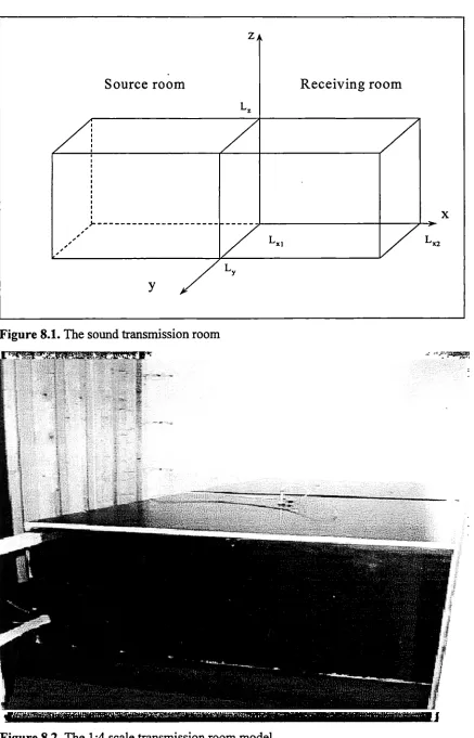
The method involves modelling the acoustic field of the two rooms as an Acoustic 1inite Element model and the displacement field of the party wall as a Structural Finite Element model. The number of elements for each model was selected by comparing the numerical eigenfrequencies with theoretical values within an acceptable processing time and error. The simulation of a single room and of two coupled rooms, defined by linking the acoustic model with the structural model, were validated by comparing the predicted frequency response with measured response of a 1:4 scale model.
The effect of three types of party wall edge condition on sound insulation was investigated: simply supported, clamped, and a combination of clamped and simply supported. It is shown that the frequency trends still can be explained in terms of the classical mechanisms. A thin masonry wall is likely to be mass controlled above 50Hz. A thick wall is stiffness controlled, below 100Hz. A clamped thin wall provides a lower sound insulation than a simply supported, whereas a clamped masonry wall provides greater sound level difference at low frequencies than a simply supported.
The sound insulation of masonry walls are shown to be strongly dependent on the acoustical modal characteristics of the connected rooms and of the structural modal characteristics of the party wall. The sound pressure level difference displays a sequence of alternating maxima and minima about a trend, dictated by the properties of the party wall. The sound insulation is lower in equal room than in unequal rooms, whatever the edge conditions and smaller wall areas provide higher sound insulation than large areas.
AKNOWLEDGEMENTS
Despite a very stormy PhD with six supervisors, four of which left the University, I
would express my gratitude to Dr. Hocine Boughdah, my director of studies, and Prof.
David Oldham of the University of Liverpool, who kindly accepted to become the first
supervisor of this present project.
I would like to acknowledge my very good friends, Marie Walker, Robin Hall, Miles
Seaton and Cinnamon Bennett, who were always there to make me laugh.
I greatly thank Garry Seiffert of the Acoustics Research Unit of the University of
Liverpool for his great help and advice for my laboratory measurements and Sid
Robinson for his excellent work on the perspex plate. I also thank Dr Andy Moorhouse
with whom I had many profitable discussions in acoustics and other interesting subjects.
Thanks also should go to Dr. John Goodchild, Dr. David Waddington, Max Fane De
Salis, Qi Ning and to all of ARU who made my life very enjoyable.
Many thanks to my family for their supports.
I greatly thank Chris who has been very patient and also very supportive all along this
PhD.
And finally, I am deeply indebted to Prof. Barry Gibbs of the University of Liverpool as
without his advice and encouragement, this thesis would not have been written.
CONTENTS
ABSTRACT 3
AKNOWLEDGEMENTS 4
CONTENTS 5
FIGURES 10
TABLES 14
GLOSSORY OF SYMBOLS 15
1 INTRODUCTION 18
1.1 REFERENCES 21
2 SOUND INSULATION OF PARTY WALLS AT LOW FREQUENCIES 23
2.1 INTRODUCTION 23
2.2 SOUND TRANSMISSION OF AN INFINITE WALL 23
2.2.1 Transmission Loss 23
2.2.2 Classical theory ofsound insulation 24
2.3 SOUND TRANSMISSION OF A FINITE WALL 27
2.3.1 Sound insulation in a diffuse field 27
2.3.2 Sound insulation when wavelength is equal to panel dimensions 28
2.4 VIBRATIONAL BEHAVIOUR OF A FINITE WALL 29
2.4.! Thin Wall 29
2.4.2 Masonry wall 30
2.4.3 Modal behaviour 31
2.4.4 Forced Vibration 33
2.4.5 Wall radiation 34
2.4.6 Damping 36
2.5.2 Experiment set up 37
2.5.3 Measurement procedure 38
2.5.4 Edge condition identfIcation 38
2.6 CONCLUSION 40
2.7 REFERENCES 41
3 SOUND FIELD IN ROOMS AT LOW FREQUENCIES 55
3.1 INTRODUCTION 55
3.2 SOUND FIELD AT LOW FREQUENCIES 55
3.2.1 Standing waves 55
3.2.2 Axial, tangential and oblique modes 57
3.2.3 Modal density 58
3.2.4 Resonant sound fields 60
3.3 DAMPiNG 62
3.4 NUMBER OF MODES REQUIRED FOR SOUND FIELD SIMULATION 63
3.5 INFLUENCE OF SOURCE POSITION 65
3.6 CONCLUSION 65
3.7 REFERENCES 67
4 SOUND INSULATION MEASUREMENT 75
4.1 INTRODUCTION 75
4.2 STANDARD METHOD 75
4.3 WATERHOUSE CORRECTION FACTOR 79
4.4 INTENSITY METHOD 81
4.5 POWER METhOD 83
4.6 SHORT TEST METHODS 84
4.7 CONCLUSION 85
5.1 INTRODUCTION 91
5.2 ANALYTICAL MODEL METhOD 91
5.3 GEOMETRIC MODELS 93
5.3.1 Ray tracing method 93
5.3.2 Image source method 95
5.4 NUMERICAL MODEL METHODS 97
5.4.1 Boundary Element Method 97
5.4.2 Finite Element Method 98
5.4.3 SYSNOISE 10I
5.5 CONCLUSION 101
5.6 REFERENCES 103
6 IMPLEMENTATION OF TRAISMISSION ROOMS MODEL 110
6.1 INTRODUCTION 110
6.2 ROOM MODEL 110
6.2.1 Introduction 111
6.2.2 Discretization "I
6.2.3 Acoustic field 113
6.2.4 Modelling 117
6.2.5 Accuracy versus Mesh Size 118
6.2.6 Estimation of the Frequency Response 120
6.3 PANEL MODEL 120
6.3.1 Introduction 120
6.3.2 Discretization 120
6.3.3 Structural field 121
6.3.4 Modelling 122
7
EXPERIMENTAL VALIDATION FOR ONE ROOM 1337.1 INTRODUCTION 133
7.2 REVIEW 133
7.3 FREQUENCY RESPONSE MEASUREMENTS 135
7.3.1 Physical scale model '35
7.3.2 Maximum Length Sequence measurements 135
7.3.3 Set up of the experiment 137
7.4 MODELLING ONE ROOM 137
7.4.1 Mesh selection 137
7.4.2 Soundfield simulation 138
7.5 FREQUENCY RESPONSE 139
7.6 CONCLUDING REMARKS 142
7.7 REFERENCES 143
8 EXPERIMENTAL VALIDATION FOR TWO ROOMS 153
8.1 INTRODUCTION 153
8.2 THEORY OF SOUND TRANSMISSION BETWEEN RECTANGULAR ROOMS 153
8.2.1 Analytical approach 153
8.2.2 Numerical approach '57
8.3 SCALE MODEL MEASUREMENT 157
& 3.1 Transmission rooms '57
8.3.2 Party wall 158
8.4 NUMERICAL MODEL 160
8.5 VALIDATION 161
8.5.1 Frequency response of the receiving room 161
8.5.2 Sound level djfference 162
SINGLE WALL 188
9.1 INTRODUCTION 188
9.2 REVIEW 189
9.3 SOUND LEVEL DIFFERENCE PREDICTION 191
9.4 EDGE CONDITIONS 192
9.4.1 Source room-party wall 192
9.4.2 Party wall - receiving room 192
9.4.3 Source room - party wall- receiving room 193
9.5 EFFECT OF ROOM CONFIGURATION 196
9.5.1 Dwellings 197
9.5.2 Symmetric rooms 199
9.5.3 Asymmetric rooms 202
9.5.4 Wall size 204
9.6 DISCUSSION 205
9.7 CONCLUDING REMARKS 207
9.8 REFERENCES 208
10 CORRECTION FACTOR FOR SOIJN]) INSULATION IN DWELLINGS238
10.1 II'4TRODUCTION 238
10.2 REVIEW 238
10.3 STATISTICAL CORRECTION FACTOR 239
10.4 DETERMINISTIC CORRECTION FACTOR 241
10.5 CONCLUDING REMARKS 245
10.6 REFERENCES 246
11 CONCLUDING REMARKS 260
FIGURES
Figure 2.1. Sound reduction index versus frequency
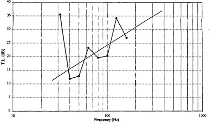
Figure 2.2 Transmission loss of a O.05m brick wall [Maluski and Gibbs (1998)]
Figure 2.3. Limit of applicability of thin plate theory to a brick wall of different
thickness
Figure 2.4. Mode (2,1) and Mode (2,2) Figure 2.5. Frequency response of a thin wall Figure 2.6. Frequency response of a thick wall
Figure 2.7. Modes (1,1), (5,3), (2,1), (3,6), (2,2), (2,4)
Figure 2.8. Radiation efficiency of the clamped and simply supported walls. Figure 2.9. Walls A and B
Figure 2.10. The transmission suite laboratory Figure 2.11. Experimental set up
Figure 2.12. Identified modes on Wall A
Figure 2.13. Identified modes on Wall B Figure 2.14. Frequency error of wall A Figure 2.15. Frequency error of wall B Figure 3.1. Room with co-ordinate system Figure 3.2. Axial modes
Figure 3.3. Tangential modes
Figure 3.4. Oblique modes
Figure 3.5. Modes with 'tails' inside the band Figure 3.6. Frequency response at low frequencies Figure 3.7. Frequency response at higher frequencies
Figure 3.8. Modal overlap
Figure 4.1. Calculated Waterhouse correction factor for the 25m3 and 50m3 rooms Figure 3.9. The reverberation time
Figure 3.10. The reverberation time at low frequencies or in small rooms Figure 5.1. Construction of the first rays reaching the receiver position Figure 5.2. Construction of the 1 and 2 order image sources
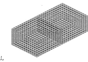
Figure 6.1. Rectangular or hexahedron elements
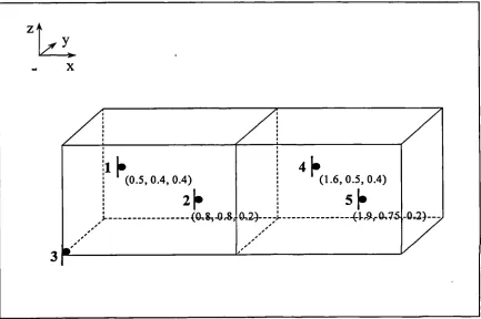
Figure 6.2. Model of the two rooms of the transmission room with co-ordinate system Figure 6.3: Acoustic model: Error versus Mode number
Figure 6.4. Acoustic model: Error versus Mode number
Figure 6.5. Frequency responses of different mesh models compared with the 11 mesh
model
Figure 6.6. Party wall
Figure 6.7. Structural model: Error versus Mode
Figure 6.8. Structural model: Error versus Mesh Model
Figure 6.9. The transmission room model
Figure 7.1. Dimensions of the 1:4 scale enclosure
Figure 7.8. Frequency response predicted at positions 1 and 2 Figure 7.9. Frequency response at microphone position I Figure 7.10. Frequency response at microphone position 2
Figure 7.11. Simulation compared with measurements in a 1/12 octave band. Figure 7.12. Simulation compared with measurements in a 1/6 octave band. Figure 7.13. Simulation compared with measurements in a 1/3 octave band. Figure 8.1. The sound transmission room
Figure 8.2. The (1:4) scale transmission room model
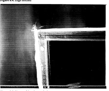
Figure 8.3. Microphone positions in the transmission rooms Figure 8.4. Edge notched
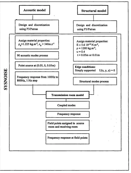
Figure 8.5. Picture of the edge notched Figure 8.6. Model of the transmission rooms Figure 8.7. Schematic of the simulation
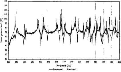
Figure 8.8. Measured and predicted frequency response of the 5mm panel at position 4 Figure 8.9. Measured and predicted frequency response of the 10mm panel at position 4 Figure 8.10. Comparison of predicted and measured sound level difference in 1/12
octave bands
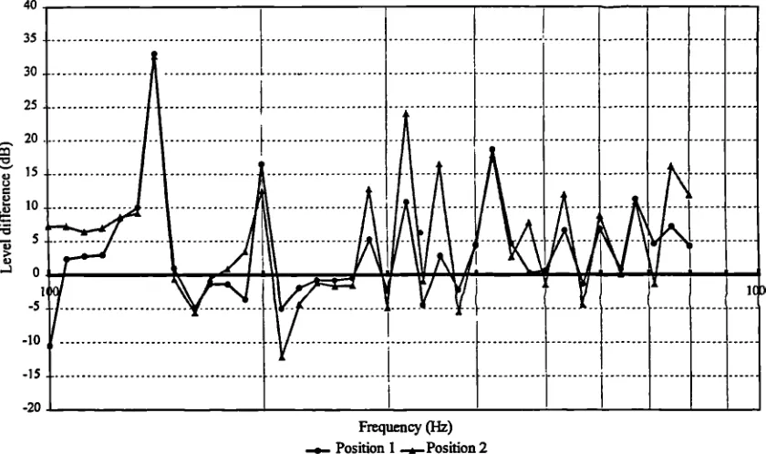
Figure 8.11. Sound pressure level difference between positions 1 and 4 of the 5mm
panel
Figure 8.12. Sound pressure level difference between positions 1 and 5 of the 5mm
panel
Figure 8.13. Sound pressure level difference between positions 2 and 4 of the 5mm
panel
Figure 8.14. Sound pressure level difference between positions 2 and 5 of the 5mm panel
Figure 8.15. Sound pressure level difference between positions 1 and 4 of the 10mm
panel
Figure 8.16. Sound pressure level difference between positions 1 and 5 of the 10 mm
panel
Figure 8.17. Sound pressure level difference between positions 2 and 4 of the 10mm
panel
Figure 8.18. Sound pressure level difference between position 2 and 5 of the 10 mm
panel
Figure 8.19. Sound level difference between positions 2 and 5 of a 5mm perspex panel in a 1/12 octave band
Figure 8.20. Sound level difference between positions 2 and 5 of a 10mm perspex panel
in a 1/12 octave band
Figure 8.21. Sound level difference between averaged positions of a 5mm panel in a
1/12 octave band
Figure 8.22. Sound level difference between averaged positions of a 10mm panel in a
1/12 octave band
Figure 8.23. Sound pressure level difference between positions 1 and 4 of a 5mm panel
in 1/3 octave bands
Figure 8.27. Sound pressure level difference between positions 1 and 4 of a 10mm
panel in 1/3 octave bands
Figure 8.28. Sound pressure level difference between positions 1 and 5 of a 10mm panel in 1/3 octave bands
Figure 8.29. Sound pressure level difference between positions 2 and 4 of a 10mm panel in 1/3 octave bands
Figure 8.30. Sound pressure level difference between positions 2 and 5 of a 10mm panel in 1/3 octave bands
Figure 8.31. Averaged sound pressure level difference of a 10mm panel in 1/3 octave
bands
Figure 8.32. Averaged sound pressure level difference of a 5mm panel in 1/3 octave bands
Figure 8.33. Positions 1 and 4: Measured sound pressure level difference compared
with predicted level difference in a 1/3 octave band
Figure 8.34. Positions 2 and 5: Measured sound pressure level difference compared with predicted level difference in a 1/3 octave band
Figure 8.35. Measured mean sound pressure level difference compared with predicted mean sound pressure level difference in a 1/3 octave band
Figure 9.1. Level difference in the source room with a 0.05m thick party brick wall Figure 9.2. Level difference in the source room with a 0.lm thick party brick wall Figure 9.3. Level difference in the source room with a 0.2m thick wall
Figure 9.4. Level difference between the clamped and the simply supported 0.05m wall
Figure 9.5. Level difference between the clamped and the simply supported 0. im wall Figure 9.6: Level difference between the clamped and the simply supported 0.2m wall Figure 9.7. Sound pressure level difference of the 0.05m wall in narrow bands
Figure 9.8. Sound pressure level difference of the 0.2m wall in narrow bands Figure 9.9. Sound pressure level difference of the 0.05m wall in 1/3 octave bands Figure 9.10. Sound pressure level difference of the 0.2m wall in 1/3 octave bands Figure 9.11. Sound pressure level difference of the 0.lm wall in 1/3 octave bands
Figure 9.12. Sound pressure level difference of the clamped 0.05m wall and simply
supported 0.lm wall in 1/3 octave bands
Figure 9.13. Sound pressure level difference of the clamped 0. Im wall and simply
supported 0.2m wall in 1/3 octave bands
Figure 9.14. Effects of edge conditions on equal room configurations
Figure 9.15. Effects of edge conditions on unequal room configurations
Figure 9.16. Effect of the edge conditions when the sound transmission direction is
interchanged. Transmission room 30-20m 3 and 20-30m3
Figure 9.17. Effect of the edge conditions when the sound transmission direction is
interchanged: 40-20m3 and 20-40m3
Figure 9.18. Effect of the edge conditions when the sound transmission direction is
interchanged: 40-30m3 and 30-40m3
Figure 9.19. Effects of room configuration on a simply supported wall Figure 9.20. Effects of room configuration on a mixed edge conditions
Figure 9.21. Effects of room configuration on a clamped wall
equal room configuration
Figure 9.27. Sound level difference of a mixed edge conditions wall when placed in different equal room configuration
Figure 9.28. Sound level difference of a clamped wall when placed in different equal
room configuration
Figure 9.29. Effects of room configuration on the sound level difference
Figure 9.30. Effects of the source room volume on the sound level difference Figure 9.31. Symmetric and asymmetric transmission rooms
Figure 9.32. Model of the asymmetric rooms configuration of 30m3
Figure 9.33. Effects of 20m3 asymmetric and symmetric equal configuration on the sound level difference.
Figure 9.34. Effects of 30m 3 asymmetric and symmetric equal configuration on the
sound level difference
Figure 9.35. Excitation of the first acoustic axial mode in the asymmetric transmission
rooms
Figure 9.36. Excitation of the first acoustic axial mode in the symmetric transmission rooms
Figure 9.37. Sound level difference of the O.2m wall of different edge conditions placed
in a 20m3 asymmetric equal room configuration.
Figure 9.38. Sound level difference of the O.2m wall of different edge conditions placed
in a 30m3 asymmetric equal room configuration
Figure 9.39. Effects of the size of the wall placed in a 20m 3 equal room configuration
on the sound level difference
Figure 9.40. Effects of the size of the wail placed in a 20m 3 equal room configuration
on the sound level difference
Figure 9.41. Size of the party wall
Figure 10.1. Standard deviation for a I 0m2 party wall placed in room configurations of
volumes smaller than 50m3
Figure 10.2. Standard deviation for the three different edge conditions of a 10m2 wall
placed between two identical rooms
Figure 10.3. Standard deviations for the three different edge conditions of the 10m2
party wall placed in unequal room (Source room volume> Receiving room volume)
Figure 10.4. Standard deviation of a 10m2 party wall of any edge conditions placed in
room configuration of volumes smaller than 50m3.
Figure 10.5. Spread and mean sound pressure level difference of a simply supported
wall
Figure 10.6. Spread and mean sound pressure level difference of a clamped wall Figure 10.7. Spread and mean pressure sound level difference of a wall
TABLES
Table 3.lumber of modes using the classical and Man's Equation
Table 3.2 Cut off frequency calculated with T = O.8s Johansson and Shi (1996)]:
Table 9.1. Number of room modes per 1/3 octave bands Table 9.2. Number of structural modes per 1/3 octave bands Table 9.3. Structural modes predicted for a brick wall Table 9.4. Typical room volumes found in dwellings Table 9.5. Room configurations
Table 10.1. Correction factor for sound level difference data of a 10m 2 party wall
Table 10.2. Correction factor for sound level difference data of a 10m 2 wall placed in
equal room configuration
TablelO.3. Correction factor for each room configuration
GLOSSARY OF SYMBOLS
A B B Bd: C C cw cccc D D1 E E F It K KN [K] [Kj L1L L1 L LL: L, L L: M [M] [Ms] N N1 N2 N [N] P Qabsorption in the receiving room (m2) bending stiffness (N.m)
bending stiffness of the plate at the notch (N.m), measurement frequency band (Hz)
kinetic energy of the sound field geometrical coupling matrix Waterhouse correction factor in dB Name given for the clamped wall
damping coefficient per unit area of the wall standardised sound pressure level difference (dB) total energy of the sound field
Young's Modulus (N.m2),
force applied on the surface of the panel transmitted intensity (W.m2)
stiffness coefficient per unit area of the wall expansion coefficient.
acoustic stiffness matrix wall stiffness matrix
space Averaged sound pressure level inside the source room (dB)
normal sound intensity (dB)
space-averaged sound pressure levels in the receiving room (dB)
length of all the edges of the enclosure (m)
spatial averaged sound pressure level inside the receiving room (dB)
power level (dB)
dimensions of the party wall (m)
dimensions of the enclosure and transmission room (m) Modal overlap
acoustic mass matrix wall mass matrix
number of eigenmodes having frequencies less than f modes of the source room of integers n,, '
modes of the receiving room of integers n,,
modes of integers ny n2 of the panel listing of shape functions
CB CL Co f t'nx,ny,nz Af S So Senci SNR ScSc SSSS T T0 T1 T.L. T.L.0 T.L.Diffuse Ux, Uy, Uz
V
surface area of the party wall (m2) S0 1 m2 a reference value
total area of the enclosure (m2) Signal! Noise Ratio
name given for the wall with mixed edge conditions simply supported/clamped/simply/clamped
name given for the simply supported wall reverberation time (s)
reference reverberation time , T = O.05s reverberation time of the source room transmission loss (dB)
transmission loss at normal incidence (dB) field incidence mass law
translational displacement in the three dimensions
room volume (m3)
V 1 volume of the source room (m3) V2 volume of receiving room (m3)
w, sound power incident (W)
W sound power transmitted (W)
Wad: radiated sound power by the wall (VT)
WR power emitted by the reference sound source (W)
W0 reference power W0 = 1 O2 (W)
['1 sound field in the source room
sound field in the receiving room
A. rotational stiffness of the plate
A' rotational stiffness in terms of the unnotched plate stiffness
primary sound field in the source room secondary sound field in the source room
'-P reverberation term
bending wave speed (m.s') longitudinal speed in wall (m.s'). sound velocity in air (m.s1) frequency (Hz)
critical frequency (Hz)
natural frequency or eigenfrequency of the structural mode
natural frequency or eigenfrequency of acoustic modes
(Hz)
12
L1 m
n(f) n , ny,, n:
Po P1 pt {p} {P}e t v (y, z)
<v211>
w
eigenvalues corresponding to g 1 in the source room eigenvalues corresponding to g2 in the receiving room width of the notch (m)
order of the sequence
model density of a bending wave field integers
sound pressure amplitude
incident sound pressure transmitted power (W)
pressure function in each element
nodal values of the pressure function associated with the element
time (s)
normal vibration velocity distribution
normal of the space time average mean square vibration velocity
vibration displacement of the wall (m)
a absorption coefficient of the surface material
C, C frequency error, error ratio(%)
volumetric strain
I Period of the Maximum Length Sequence
11 loss factor of the party wall
incident acoustic wavelength (m) critical wavelength (m)
trace wavelength (m) bending wavelength (m)
V Poisson ratio.
0 angle of incident sound wave
Ps surface density (kg.m2),
p0 air density (kg.m3)
grad radiation efficiency
transmission coefficient of the party wall
1) pressure velocity
(1) angular frequency (rad.s1).
Party wall velocity.
ö (x) Dirac function
1
INTRODUCTION
The last 50 years have shown a devel6ping understanding of the sound transmission
phenomena in dwellings [Kihiman (1991)]. This has been accompanied by an increasing
requirement for high sound insulation for party walls and floors. More recently, the
rapid development in mechanical and electrical domestic appliances has resulted in
increasing numbers of domestic noise-related complaints [Brooks (1989), Murray
(1995), Grimwood (1997)], which is also due to an increase in noise environmental
awareness. Many of the complaints are due to the low frequencies originating, for
example, from hi-fis, televisions and home-cinemas. Their frequencies often are below
100Hz [Brooks (1989), Mathys (1993), Leventhall (1995), Grimwood (1995 & 97)].
They are well above background noise and are not well controlled by the separating
walls and floors between dwellings. Moreover, such noise, including infra-sound, can
affect the health of the occupant [Berglung et al (1996), Mirowska (1997)]. Good sound
insulation at low frequencies, therefore, is an important requirement in dwellings.
Laboratory measurements of sound insulation at low frequencies produce a poor
repeatability [Farina (1997)]. Repeatability is qualitatively, the closeness of agreement
between successive results obtained with the same test procedure on the same test
specimen under the same conditions (same operator, apparatus, laboratory and short
intervals of time between tests) [ISO 140 part 2 (1993)]. Measurements of sound
insulation at low frequencies are also known to produce a poor reproducibility [Roland
(1995), Goydke (1998)]. Reproducibility is qualitatively, the closeness of agreement
between individual results obtained with the same method on identical test specimens
but under different conditions (different operators, different apparatus, different
laboratories and different times) [ISO 140 part 2 (1993)]. Recent investigations have
shown that repeatability and reproducibility in laboratories can be improved by placing
special absorption panels [Fuchs et a! (1998)] at positions which correspond to acoustic
measurements at low frequencies also have poor repeatability and poor reproducibility.
The problem, stated in Chapters 2 and 3, is that the classical theory of sound fields and
sound insulation and the measurement procedures and corrections which result from
them, are not relevant to low frequencies. The theory does not apply when the sound
wavelength is large compared with room and wall dimensions, and must be replaced
with a modal characterisation of the sound field and of the wall vibration. A room mode
or a structural mode is defined as an acoustic or a structural wave which travels along a
path and comes back at its starting point.
Present methods of measurements of sound insulation are described in Chapter 4. It is
confirmed that the methods of measurement and rating of walls and floors are tenuous
below 100Hz.
Measurements of the vibrational field on typical brick walls, presented in Chapter 2,
show that the wall edge conditions have a strong effect on the modal behaviour and
therefore on the sound insulation at low frequencies. The need to include the edge
conditions in the study is highlighted.
The core of this thesis is an investigation of the sound transmission between dwellings
in the frequency range 25 - 200Hz. Since no accurate method is available for low
frequency measurement, various methods of predicting the sound fields and the wall
vibrations are described in Chapter 5 to find the best method.
A Finite Element Method (FEM) is proposed. The theories of the acoustic finite element
and of the structural finite element methods are described in Chapters 6 and 8. Its
implementation is described in Chapter 6, in particular, the number of elements required
to model the rooms and party wall, accurately.
To use FEM for subsequent studies, the choice of the mesh models is validated in
by a party wall, as described in Chapter 8. A Structural - Acoustic Finite Element model
is created and is validated by comparing the predicted and measured sound pressure
level differences. FEM is shown to be an appropriate method for predicting sound
transmission at low frequencies between rooms of volumes less than or equal to 50m3.
A parametric survey is conducted of the effects of edge conditions and room
configuration on the sound level difference in Chapter 9. The effects of edge conditions
and room configuration are studied.
In Chapter 10, an attempt is made to find a form of correction factor to field level
difference from the deterministic and statistical survey.
1.1 REFERENCES
Bergland, B. and Hassmen, P., (1996): 'Sources and effects of low frequency noise',
Journal of the Acoustical Society of America, Vol.99 (5), 2985-3002
Brooks, J. R., Attenborough, K., (1989): 'The implication of measured and estimated
domestic source levels for insulation requirements', Proceeding of I.O.A., Vol.11
(11), 19-27
Farina, A., Fausti, P., Pompoli, R. and Scamoni, F., (1997): 'Intercomparison of
laboratory measurements of airborne sound insulation of partitions pompoli',
Proceeding of Inter-Noise 97, 881-886
Fuchs, H.V., Zha, X., Spah, M. and Pommerer, M., (1998): 'Qualflcations of small
freefield and reverberation rooms for low frequencies', Proceeding of Euro-Noise
98, Vol.2, 65 7-662
Goydke, H., (1998): 'Investigations on the precision of laboratory measurements of
sound insulation of building elements according to the revised Standard ISO 140
Proceeding of Inter-Noise 98, 480
Grimwood, C., (1995): 'Complaints about poor sound insulation between dwellings',
Bulletin of the Institute of Acoustics, Vol.20 (4), 11-16
Grimwood, C., (1998), 'Occupant opinion of sound insulation in converted and
refurbished dwellings in England and the implication for national building
Regulations', Proceeding of Euro-Noise 98, Vol.2 (2), 705-7 10
ISO 140 (1978): 'Measurement of sound insulation in buildings and building elements
Part 2: Statement ofprecision requirements'
Kihiman, T., (1991): 'Fifty years of development in sound insulation of dwellings',
Proceeding of Inter-Noise 91, 3-15
Knudsen, V.0., (1932): 'Resonance in small rooms', Journal of the Acoustical Society,
July 1932, 21-37
Leventhal, H.G., (1995): 'The role of low frequency noise and infrasound in sound
results and assessment ofannoyance', 5t1 International Congress on Sound and
Vibration, 15-18 December, Adelaide, South Autralia
Murray, I., (1995): 'Noisy neighbours', Journal THE TIMES, Monday 14 August
1995, 1-7
Pedersen, D.B., (1997), 'Laboratory measurement of the low frequency sound
insulation', DAGA 97, Kiel, 105-106
Roland, J, (1995): 'Adaptation of existing test facilities to low frequencies
2 SOUND INSULATION OF PARTY WALLS AT LOW
FREQUENCIES
2.1 INTRODUCTION
In Chapter 1, it has been highlighted that airborne sound insulation is difficult to
measure at low frequencies. In this chapter, it is shown that classical theories of sound
fields in enclosures and the transmission of sound through panels are not applicable
because the modal behaviour of the sound fields and of the panel are not described. This
will be demonstrated by first describing sound insulation of an infinite wall using
classical theory. Then, sound insulation of a finite wall is described for both diffuse and
non diffuse sound fields. The modal behaviour of the party wall and of the sound field
will be observed to control the sound transmission. Measurements of the structural
modes of two brick walls are described and the effects of edge conditions are observed
to control the eigenfrequencies, and hence the bending wave modal distribution.
2.2 SOUND TRANSMISSION OF AN INFINITE WALL
2.2.1 Transmission Loss
In classical theory, the wall is assumed thin, isotropic, flat and infinite in extent
[London(1949), Sewell (1970), Beranek (1992), Bies et al (1996)J. An incident sound
wave strikes the surface of the wall at an angle 0. Part of the sound energy is reflected,
part of it is absorbed and part of it is transmitted. The determination of the energy
transmitted through the wall is defined by the transmission coefficient 'r, given [Beranek
where t (0,0)) is the transmission coefficient of the party wall at incident angles 0 and
angular frequency (1), wine (e,) is the sound power incident on the source side and
Wtrs(e,cI)) is the sound power transmitted to the receiver side.
The transmission can be expressed in terms of the transmission loss (T.L.) in dB, also
known as the sound reduction index (R), given by;
T.L. = 10 log1 (2.2)
2.2.2 Classical theory of sound insulation
The sound insulation is often described by the approximate equation [Crocker et a!
(1982)];
T L io1og[D +(ps
= 4pc/cos2O
J
(2.3)
where D = D + 2p0 c 0 /cosO, D is the damping coefficient per unit area, K is the stiffness coefficient per unit area, Ps is the mass per unit area, p0 is the air density,
c 0 is sound velocity in air. Equation 2.3, however, does not include the effects of the
higher order panel resonances and wave coincidence, which have been observed
experimentally.
The transmission loss against frequency, presented in Figure 2.1, is deduced partly from
theoretical and experimental considerations. Five regions are distinguished:
K/w
T.L.=1Olog 222 j (2.4)
The sound transmission loss decreases with frequency increase, at -6dB/octave,
until the first panel resonance is excited [Bies et al (1996)]. Transmission loss is
dependent on the incident angle and the medium fluid.
2. Wall resonance
The wall resonates at frequencies where the mass and the stiffness controlled
mechanisms cancel. This phenomenon is described in detail in section 2.4.2.
3. Mass control
The sound transmission is controlled by the mass of the wall, according to;
TL 10lo[_()))
2
4pc /cos2 9J
(2.5)
where the terms are as in Equation 2.3. The wall in this region behaves as a limp
wall. K and D are negligible. The transmission loss also depends on the angle of
incidence, e.
For normal incidence, when 0 0,
T.L. 0 =20 log
I_
2p0c0Also, if the wave strikes the wall at grazing incidence (0 =900), the sound is
If all incident angles are included to give a random incidence value, the Equation
2.5 is rewritten as follows;
T •L•RafldOm =T.L. 0 -10 log (0.23 T.L. 0 ) (2.7)
If angles from the normal to 78° are included (T.L. 0 >15dB), the Equation 2.7
becomes [Berariek (1992)];
T.L. DISC = T.L. 0 -5 (2.8)
where T.L. Diffiise is known as the field incidence mass law
4. Coincidence region
The coincidence region starts from the critical frequency, when the bending
wave speed (see Section 2.4.1) equals the sound speed.
When the wall is excited by an incident acoustic wave, A., at an angle 9, a trace
wave of wavelength ?, is generated, where
T=?I /sinO (2.9)
When the trace wavelength matches free bending wavelength, 'b, wave
coincidence occurs and Ab =X1/ sin 0. Critical coincidence takes place at grazing
incidence (i.e. 9 =0). Subsequent wave coincidences occur at non-grazing angles,
up to the damping control region.
5. Damping control
The sound transmission is controlled by the damping of the wall, which is mainly
due to the transfer of energy through the junctions to other parts of the buildings
where ii is the loss factor of the party wall. In this region, the transmission loss
increases at 9dB per octave till the mass law performance is recovered at
6dB/octave.
2.3 SOUND TRANSMISSION OF A FINITE WALL
2.3.1 Sound insulation in a diffuse field
An isotropic wall of dimensions greater than the incident sound wavelength is
considered. Bending wave resonances are allowed at specific frequencies, dictated by
the wall dimensions. However, the predicted transmission loss for infinite walls often
applies to finite walls. The sound pressure level on the source side, L 1 , forces the panel
to vibrate, which then radiates to the receiving side creating a sound pressure level, L2.
The transmission loss is then obtained from the two sound pressure levels, the surface of
the party wall, S, and the absorption in the receiving room, A, giving;
T.L.=L 1 —L 2 +1Olog(-) (2.11)
Such relationships are however only applicable for frequencies well above the first
bending-wave resonance of the panel where the wavelength is small compared with the
party wall dimensions [Bhattacharya (1971)]. The edge conditions are assumed not to be
influential, whereas the real edge conditions of the party wall are found to have a strong
influence on the coincidence region [Kihlman (1970), Kihlman (1972), Bies et al
(1996)]. The coincidence region tends also to be not observable when the thickness of
the party wall is large such as for masonry walls [Bergasolli (1970)]. The damping
region is strongly influenced by edge damping and internal damping. Despite those
2.3.2 Sound insulation when wavelength is equal to panel dimensions
The same thin, flat, isotropic wall is considered. The sound wavelength, now, is equal or
greater than the panel dimensions. Two types of sound pressure fields are considered:
1) The sound field consists of a large number of excited room modes in the
measurement band (often one-1/3 octave). An example of this is the sound fields
in large rooms at low frequencies
2) The sound field consists of a small number of excited room modes. An example of
this is the sound fields in small rooms.
In the first case, the sound transmission loss deviates from the mass law, whatever the
panel dimensions [London (1949), Sewell (1970), Nilsson (1972), Mulholland (1973),
Novikov (1998), Gargliadini (1990-91)]. The panel radiates like a piston [FleckI (1981)].
Nilsson [1972] defmed a new relationship which takes into account the non-statistical
behaviour of the sound field and the modal behaviour of the panel, including edge
conditions. Novikov [1998] defined a correction factor including the area of the plate
and of the laboratory wall where the panel is placed. Utley [1968] and others [Nilsson
(1972), Bhattacharya (1972)] showed that the discrepancies depend on the configuration
of the transmission rooms (dimensions, aspect ratio, etc.).
The second case is illustrated by Figure 2.2. The transmission loss shows the same trend
as a mass law trend, but displays alternating maxima and minima due to acoustic
couplings between rooms. The phenomenon has been observed by many authors [Heckl
(1958), Utley (1968.), Muiholland (1973), Sharp (1978), Kropp (1994), Osipov
(1996-97), Pietrzyk (19(1996-97),]. The number of excited room modes is much less than that in a
diffuse sound field and the sound is transmitted by forced vibration of the wall [Josse
and Lamure (1964), Sharp (1978)]. The room modes force the surface of the wall to take
the same mode shape which then radiates into the receiving room. These strong
variations tend to cancel each other out when 20 modes at least are excited in a third
Pietrzyk (1997)]. Again, the sound is transmitted by forced vibration of the wall [Josse
and Lamure (1964), Sharp (1978)]. Acoustic-structural couplings occur, which also
create alternating maxima and minima in transmission loss. The forced transmission is
seen as the most important phenomenon of transmission rather than the transmission at
resonance [Josse and Lamure (1964), Muiholland (1973)].
To suminarise, the transmission loss at low frequencies is strongly influenced by both
the acoustical and the structural modal characteristics.
2.4 VIBRATIONAL BEHAVIOUR OF A FINITE WALL
2.4.1 Thin Wall
A finite wall is assumed where thickness is small compared with the airborne and
structure borne wavelengths. Various structural waves are generated when a force is
applied to the surface of the wall or a force applied to all surfaces [Fahy (1985)]. They include shear, torsional and compressional waves. Shear waves are identified as
transverse waves with displacements normal to the plane of the wall. Torsional waves
are also shear waves, but are characterised by a torsional displacement. The direction of
particle displacement of compressional waves is in the direction of wave propagation.
The three waves are regrouped into one flexural wave; the bending wave which depends on the thickness of the wall. A wall cannot be considered as thin when the thickness is
greater than a sixth of the bending wavelength [Cremer (1953 & 88)].
The bending stiffness, B, is defmed as follows;
B=_Eh3
Bending waves control the surface displacement of the wall. They are easy to excite due
to their low input impedance, and are good sound radiators because their motion is
normal to the plate surface.
Bending wave speed, CB, is given by;
i
1/2CB=I (m.s1) (2.13)
L
Ps)where Ps is the surface density of the wall (kg.m2)
The speed of the bending wave increases with the square root of the frequency. It is
dependent upon the thickness of the wall, where the lowest propagation speed is
obtained for the thinnest wall. The bending wave speed is smaller than the velocity of
sound in air at frequencies below the critical frequency and greater above the critical
frequency. Such differences in velocity explain the radiation and control of the sound
transmission through the wall.
2.4.2 Masonry wall
When a thick wall i.e. a wall with a thickness greater than 116 of the bending
wavelength, is excited by an acoustic wave, bending waves and shear waves are excited.
Resonance and radiation efficiency are then different from a wall where only bending
waves are excited [Heckl (1958 & 81), Llungren (199 1-a&b), Rindel (1988)].
Rindel {1988] developed an expression for wall radiation, which combines the bending
wave and shear wave speeds. He showed that at low frequencies, speed of transverse
waves is asymptote to the bending wave speed. The wall radiation is therefore
controlled by the bending wave speed only. Liungren [1991] investigated analytically
k+k2 i,.2 ...(w2p z lB)" 2 (2.16) That idea, however, is not developed here. Consequently, the thick wall can be
expressed by the classic thin plate theory [Cremer (1953 & 88)].
A brick wall of 0.125m thickness in section 2.5 and three other brick walls of 0.5, 0.1 and 0.2m thickness in Chapter 9 are investigated. The limit of applicability of the thin
plate theory to a 0.5m brick wall of longitudinal velocity equals to 2350Hz is shown in
Figure 2.3 [Cremer (1953 & 88)1. The thin plate theory can only be applied below 2475Hz. For a brick wall of 0.lm, 0.125m and 0.2m thickness, the thin plate theory is
only applicable below 1236Hz, 996Hz and 619Hz, respectively. As the frequency range
of interest is 25Hz - 200Hz, thin plate theory can apply.
2.4.3 Modal behaviour
The vibration displacement w of the fmite wall [Fahy (1985), Leissa (1993)] is
expressed as;
(2w ö 2 w 2 (a2w Bi--i- i =-pi
öy 2 z2)
where t is the time.
A solution of this equation is
w(y,z,t)= exp[j(wt - ky - kz)J
where
(2.14)
(2.15)
kb is the free bending wavenumber and lc, k are the wavenumber components in the
v(y,z), takes the form
•
. (,rnz'\
v(y,z)=vnynz sin L) Isin' L)I (2.17)
rn rn
k Y
forO^y^L,O^z^L,n,nareintegersand
=
k=—--Substituting lc and k into Equation 2.16, the natural frequencies of a simply supported
wall is given by [Warburton (1953), Leissa (1993)]
( \1/21( \2 B II fl I
=-
;J
[J
L)](2.18)
is also called the eigenfrequency of the structural mode, identified by the integers
n and n. Those modes occur when the structural wave reflects to form a standing wave.
Standing waves can be identified by the presence of points or lines of zero
displacement, called nodes, and areas of maximum displacement, called anti-nodes. The
modal pattern at an eigenfrequency is identified by the integers n, and ny.
Two types of mode shape can be identified. The first is when the flexural wave only
propagates in one dimension e.g. n,,, = 1. The second is when the structural wave
propagates in two dimensions. Those structural modes are dependent on the frequency
and the wall dimensions [Warburton (1953), Leissa (1993)]. Figure 2.4 shows one
dimensional and two dimensional modes.
When the excitation frequency coincides with the natural frequency of the plate [Fahy
(1985)], the panel is said to be resonant and can lead to a reduction in transmission loss.
The number of modes and the mode shapes vary with the panel dimensions. The number
of modes also differs between thin and heavyweight walls. Figure 2.5 shows the number
of modes for a thin plate, while Figure 2.6 shows the number of modes for a
heavyweight wall.
For the thin plate, the first structural mode is excited at low frequency. The mode
density of a bending wave field, n(f), is independent of frequency and is given by
[Beranek (1992)];
_
Ts
n(f)= = ________ s (2.19)
2cLh
2' E h
p(l-v2)
where CL is the longitudinal speed (m.․ )
For a thick wall, the first structural mode is excited higher in the frequency range and
the modes are well spaced.
Modification of the dimensions changes the modal density and the mode shape, and
therefore influences the sound transmission loss [Gargliadini (1991)]. However, those
effects tend to be reduced when at least 3 modes per third octave bands are excited.
2.4.4 Forced Vibration
The response of the wall varies if the excitation is localised (e.g. a hammer) or extended
(e.g. airborne sound). When excited by a localised force, the position of the excitation
can be on a nodal line of zero displacement or at an anti-node of maximum
displacements. If on the nodal line, the wall cannot be excited. Thus, the applied force
wall surface to take the same mode shape as the acoustic mode.
2.4.5 WaIl radiation
When the incident sound field drives the wall, free and forced vibrations take place. The
air particle motion, normal to the vibrating surface, tends to cancel over a bending
wavelength, in the middle of the wall surface. However, at boundaries, the cancellation
is not total and radiation occurs. Therefore, radiation is strongly dependent on the ratio
of the bending wavelength to that in air.
For a wall of dimensions greater than the acoustic wavelength, resonant modes can be
classed as either acoustically fast (A.F.) modes or acoustically slow (A.S.) modes
[Crocker (1982)]. The A.F. modes correspond to wavelengths greater than the acoustic
wavelength. They always match the trace wavelength and the fluid cannot produce
pressure waves which will move fast enough to cause any cancellation. The wall thus
radiates from the whole surface area of the wall, giving a high radiation efficiency.
The A.S. modes correspond to wavelengths smaller than the acoustic wavelength. The
fluid produces pressure waves which move fast enough to cause cancellation. The
radiation efficiency is low. The radiation is first the result of A.S. modes at plate corners
where cancellation is incomplete. At higher frequency, edge modes occur where the
bending wave speed is subsonic only in a direction parallel to one pair of edges and
supersonic in a direction parallel to the other pair. Cancellation can only occur in one
edge direction.
When modes are not vibrating at their resonance frequencies, little sound is radiated and
there is poor coupling between the wall and the fluid. The sound transmission is termed
non resonant and gives rise to the mass law transmission.
own radiation efficiency 0rad defined as
0rad =
<v > p0c0S
(2.20)
where <v> is the normal of the space time average mean square vibration velocity of
the radiating surface of area S and W d is the radiated sound power.
The odd-odd modes (e.g. modes (1,1), (5,3)) are found to radiate more than the
even-odd modes (e.g. modes (2,1), (3,6)) and even more than the even-even modes (e.g.
modes (2,2), (2,4)) [Schroter et a! (1981), Fahy (1985)]. It can be explained by looking
at the number of positive and negative cells seen in Figure 2.7. When cells situated on
the opposite sides of the wall are of the same sign, the wall radiates more than that with
cells of opposite sign. The radiation is also controlled by the surface of the cell. If there
are many cells i.e. cells of small area, cancellation occurs reducing the amount of
radiated energy.
The radiation efficiency of a mode can be altered with the force applied on the surface
of the wall [Simmons (1989)]. Indeed, the wall surface can be forced to take the same
shape as its eigenmode at any frequency. The radiation of the wall is then the sum of the
radiation efficiencies of all the modes.
Radiation efficiency is dependent on the dimensions of the wall {Schroter et al (1981),
Novak (1994)]. Low radiation efficiency is obtained for plates which are less than 16m2
and the critical frequency is not observed [Novak (1994)]. Radiation efficiency is
dependent on the thickness of the wall [Schroter (1981), Lamancusa (1994)] and
variable thickness can lead to minima in sound radiation [Lamancusa (1994)]. Radiation
efficiency is dependent on the edge conditions as seen in Figure 2.8 [Maidanik (1962),
2.4.6 Damping
The damping may take the form of material damping, interface damping, or radiation
into connected fluids. In most cases, damping does not significantly change the phase
velocity and has not much effect in the sub-critical region of the party wall [Fahy
(1985)1, but is effective when the response of the panel is dominated by resonant modes.
Resonant and coincidence regions are controlled by damping.
2.4.7 Edge Conditions
The two extreme wall edge conditions are simply supported and clamped. Simply
supported allows no transverse displacement and produces shear force reaction, but
rotational movement is not restrained. Clamped edge condition allows no transverse or
rotational displacement. The change of edge conditions from simply supported to
clamped condition results in a shift of the structural modes to higher frequencies
[Warburton (1953), Cremer (1988)]. The modal pattern and thus the radiation of the
wall is then modified [Warburton (1953), Maidanik (1970), Sewell (1970), Kihiman
(1970), Nilsson (1972), Berry et al (1991), Guyader et al (1994), Lamancusa (1994)].
This in turn alters the transmission loss [Balike (1994), Berry et al (1994)].
When the wall is excited by an acoustic wavelength smaller than the panel dimensions,
clamped conditions lead the thin plate to radiate twice the energy of the simply
supported condition [Maidanik (1962), Sewell (1970), Kihlman (1970), Nilsson (1972)].
To summarise; edge conditions control the forced and free bending waves and thus the
transmission loss.
modal density, with a first eigenfrequency high in the frequency range. Also in section
2.4.7, it was highlighted that edge conditions control the modal density. It is therefore
necessary to investigate experimentally the edge conditions of real walls as a prelude to
investigating vibro-acoustic coupling in Chapter 9. It is not likely that the edge
conditions of masonry walls are properly described as simply supported, clamped or any
other classical condition. Therefore, the vibration response of typical brick walls was
measured from which the installed edge conditions could be inferred.
2.5.1 Two Brick walls
Two brick walls of a transmission suite were chosen for this experiment as seen in
Figure 2.9. The larger wall, A, was of dimensions 2.88 x 2.49m. The smaller wall, B,
was 1.84 x 2.49m. Both walls were of 115mm brick, with one side painted and the other
side covered with a plaster layer (internal face). Both were supported by a concrete slab
with a concrete ceiling on the top (see Figure 2.10). The walls formed two junction
types. The first was with the floor and the roof slab. The second formed a corner with
the other brick walls.
2.5.2 Experiment set up
Figure 2.11 illustrates the experimental set up for measuring vibrational response. The
measuring system comprised of an electro-dynamic shaker, a function generator, a
power amplifier, two accelerometers, a charge amplifier and an oscilloscope.
The position of the shaker on each wall was chosen carefully to ensure that it was not at
a structural node. According to Equation 2.18, modes (1,2), (2,1), (3,1), (1,3), (2,2), are
likely to be excited below 200Hz. The corresponding nodal lines are along the centre of
the walls or at a distance of one third dimensions from the edges. Therefore the shaker
I n - +0.25 +1
L (2.21)
bolting it in order to reduce the influence of local defonnation.
2.5.3 Measurement procedure
The power amplifier and function generator were used to drive the electro-clynamic
shaker with a slow swept sine signal over 0-200Hz. The signal sent to the shaker was
shown on the oscilloscope and used as a reference. An accelerometer was used to record
the acceleration amplitudes of the surface at points on a O.300m x O.355m grid for wall A and on a O.300m x O.250m grid for wall B. The signal from the accelerometer also
was displayed on the screen of the oscilloscope and compared visually with the
reference signal. The nodal lines were determined when the measured signal was a
minimum or when the measured signal changed phase with respect to the reference
signal. It was possible to identify several lower order modes as shown in Figures
2.12-13. Modes (1,1), (2,1), (3,1) and (1,3) of wall A (see Figure 2.12) and modes (1,1),
(1,2), (2,1), (2,2) and (1,3) of wall B (see Figure 2.13) were obtained. The measurement
of modes shapes was relatively easy at very low frequencies, but became more difficult
as the frequency increased, particularly, the mode (1,3) of wall A.
2.5.4 Edge condition identification
In order to identify the likely corresponding edge conditions, the eigenfrequencies and
their order were compared with theoretical prediction according to Warburton [1953]
and Leissa [1993].
For a simply supported panel, the resonance frequencies are calculated from Equation
2.18. An approximate expression is given for a rectangular supported panel having one
clamped edge [Leissa (1993)];
2r BI(n
and for a rectangular supported panel having two clamped edges [Leissa (1993)];
=i[[]2
(n,_o•52 +1
-t L (2.22)
As the wall properties were not known, the factor including bending stiffness and mass
surface was defined using the wall dimensions and the measured eigenfrequency of the
first mode. The other theoretical eigenfrequencies were then calculated. That means the
clamped conditions cannot be calculated as the relationship not only depends on that
factor but also depends on Poisson's ratio value. The clamped condition was therefore
not calculated.
Figure 2.14 and Figure 2.15 show the frequency error s, calculated between the theoretical and measured eigenfrequencies of the wall A and B, respectively, for simply
supported, simply supported with one clamped edge, and simply supported with two
clamped edges, according to the following relationship;
Predicted value - Measured value xlOO
Predicted value (2.23)
The smallest error for each mode was obtained for two simply supported and two
clamped edges, whatever the wall.
In general, the edge conditions of a real party wall therefore lie between simply
supported and clamped, a phenomenon already observed by Balike [1994]. However,
the two walls have corner edges which often is not present in constructions of dwellings.
Real party walls have T-edges, and they provide stiffer edge constraint than corner
edges. The approach of this study therefore was to investigate the range of possible edge
2.6 CONCLUSION
Classical theory of sound insulation does not apply when the sound field is not diffuse
and when the party wall has only a few structural modes in the frequency range of
interest. The transmission loss is governed by the interaction of the acoustic and the
structural modes. Thus any modification to the structural modal distribution will
influence the transmission loss. The structural modal distribution is dependent on wall
dimension and edge condition and in real buildings, those two factors are likely to vary
significantly.
Measurements have shown that the real edge conditions of a brick wall are likely to lie
between simply supported and clamped. Consequently, the sound transmission loss at
low frequencies can only be predicted by taking account of the acoustical modal
behaviour of the source and receiving rooms and of the structural modal behaviour of
the party wall including the edge conditions. The acoustic field in rooms nov vii\\ be
2.7 REFERENCES
Balike, M. and Bhat, R.B., (1994): 'Noise transmission through a cavity backed
flexible plate with elastic edge constraints', 3rd International Congress on Air and
Structure Borne Sound and Vibration, 335-343
Beranek, L.L. and Ver, I.L., (1992): 'Noise and Vibration Control Engineering:
Principles and Applications', Ed. J.Wiley and Sons
Bergassoli, A. and Brodut, M., (1970): 'Transparence des murs et des cloisons',
Acustica, Vol.23, 3 15-322
Berry, A. and Guyader, J.L., (1991): 'A general formulation for the sound radiation
from rectangular baffled plates with arbitrary boundary conditions', Journal of
Acoustical Society of America, Vol.37 (5), 93-102
Berry, A. and Nicolas, J., (1994): 'Structural acoustics and vibration behaviour of
complex panels' , Applied Acoustics, 'Vol.43, S-2X5
Bhattacharya, MC. and Guy, R.W., (1972): 'The influence of the measuring facility
on the measured sound insulating property of a panel', Acustica, Vol.26, 344-348
Bhattacharya, M.C., Guy, R.W. and Crocker, M.J., (1971): 'Coincidence effect with
sound waves in a finite plate', Journal of Sound and Vibration, Vol.18 (2),
157-169
Bies, D.A. and Hansen, C.H., (1996): 'Engineering noise control: Theory and
practice', 2nd Ed. E & FN SPON
Craik, R.J.M., (1981): 'Damping of building structures', Applied Acoustics, C.8 1,
347-359
Cremer, L., (1953): 'Calculation of sound propagation in structures', Acustica, Vol.3
(5), 3 17-335
Cremer, L., Heckl, M. and Ungar, E.E., (1988): 'Structure-Borne Sound', Ed.
Springer-Verlag
Crocker, M.J. and Kessler, F.M., (1982): 'Noise and Noise Control', Vol.2, Ed. Crc
acoustic transmission between rooms', Journal of Sound and Vibration, Vol.145
(3), 457-478
Gargliadini, L., (1990): 'Simulation numerique de la mesure en laboratoire de l'indice
d'affaiblissement acoustique. Effets des sources et de la geometrie de la paroie',
Colloque de Physique, Colloque C2, Supplement n° 2, Tome 51
Gibbs, B.M. and Gilford, C.L.S., (1976): 'The use of power flow methods for the
assessment of sound transmission in building structures', Journal of Sound and
Vibration, Vol.49 (2), 267-286
Guyader, J.L. and Laulagnet, B., (1994): 'Structural acoustic radiation prediction:
Expanding the vibratory response on a functional basis', Applied Acoustics,
Vol.43, 247-269
Halliwell, R.E. and Warnock, C.C., (1985), 'Sound transmission loss: Comparison of
conventional techniques with sound intensity techniques', Journal of Acoustical
Society of America, Vol.77 (6), 2094-2103
Hecki, M. and Seifert, K., (1958): 'Investigations f the influence of eigen-resonances
of rooms on the result of the sound insulation measurement', Acustica, Vol.8 (4),
212-220
Hecki, M., (1981): 'The tenth Sir Richard Fayrey memorial lecture: sound transmission
in buildings', Journal of Sound and Vibration, Vol.77 (20), 165-189
Josse, R. and Lamure, C., (1964): 'Transmission du son par une paroie simple',
Acustica, Vol.14, 267-280
Kihiman, T., (1967): 'Sound radiation into a rectangular room. Application to
airborne sound transmission in Buildings', Acustica, Vol.18, 11-20
Kihiman, T., (1970): Report on the influence of boundary conditions on the reduction
index, Report NO ISOITC43/SC2/WG2, Chalmers Tekniska Hogskila, Goteborg,
Sweden
Kihiman, T and Nilsson, A.C., (1972): 'The effects of some laboratory designs and
mounting conditions on reduction index measurements', Applied Acoustics, Vol.5
Kropp, W., Pietrzyk, A. and Kihiman, T., (1994): 'On the meaning of the sound
Ljunggren, S., (1991-a): 'Airborne sound insulation of thin walls', Journal of
Acoustical Society of America, Vol.89 (5), 2324-2337
Ljunggren, S., (1991-b): 'Airborne sound insulation of thick walls', Journal of
Acoustical Society of America, Vol.89 (5), 2338-2345
London, A., (1949): 'Transmission of reverberant sound through single walls',
Research Paper RP1998, Vol.42, 605-615
Maidanik, G., (1962): 'Response of a ribbed panels to reverberant acoustic fields'
Journal of Acoustical Society of America, Vol.34, 809-826
Maluski, S. and Bougdah, H., (1997): 'Predicted and measured low frequency
response of small rooms', Journal Building Acoustics, Vol.4 (2), 73-86
Maluski, S. and Gibbs, B.M., (1998): 'The influence ofpartitions boundary conditions
on sound level dfference between rooms at low frequencies', Proceeding of
Euro-Noise 98, Vol.2, 68 1-686
Muholland, K.A. and Lyon, R.H., (1973): 'Sound insulation at low frequencies',
Journal of Acoustical Society of America, Vol.54 (4), 867-878
Nilsson, A.C., (1972): 'Reduction index and boundary conditions for a wall between
two rectangular rooms, Part land II', Acustica, Vol.26, 1-23
Novak, R. A., (1994): 'The radiation factor offinite plates at low frequencies', Third
International Congress on Air-and structure-borne sound and vibration, June
13-15, Montreal, 23-29
Novikov, I.!., (1998): 'Low-frequency sound insulation of thin plates', Applied
Acoustics, Vol.54 (1), 83-90
Osipov, A., Mees, P. and Vermeir, G., (1996): 'Low frequency airborne sound
transmission in buildings: Single plane walls', Proceeding of Inter-Noise 96,
1791-1794
Osipov,A., Mees, P., and Vermeir, G., (1997): 'Low frequency airborne sound
transmission through single partitions in Buildings', Applied Acoustics, Vol.52
(3-4), 273-288
Schroter, V. and Fahy, F.J., (1981): 'Radiation from modes of rectangular panel into
a coupled fluid layer', Journal of Sound and Vibration, Vol.74 (4), 575-5 87
Sewell, E.C., (1970): 'Transmission of reverberant sound through a single leaf
partition surrounded by an infinite rigid baffle', Journal of Sound and Vibration,
Vol.12 (1), 21-32
Sharp, B.H., (1978): 'Prediction methods for the sound transmission of building
elements', Noise Control Engineering, September- October 1978, Vol.11(2),
53-62.
Simmons, C. and Maxwell, R., (1989): 'Radiation index of baffled plates with
stffeners, using the finite element method and the fast fourier transform',
Proceeding of Inter-Noise 89, 530-534
Utley, W.A., (1968): 'Single leaf transmission loss at low frequencies', Journal of
Sound and Vibration, Vol.8 (2), 256
Warburton, G.B. (1953): 'The vibration of rectangular plates', Proceeding of. Onst.
Bending
stiffness
control
Mass
law.
control
C')
Damping
Coincidence control
region
Cl,
Cl,
0
0
Cl)
Cl)
fi f2
100 1000
Freqtncy (Hz) 40
35
30
25
20
I.-15
I0
5
0 10
[image:46.595.75.508.393.654.2]Frequency (Hz)
Figure 2.1. Transmission loss versus frequency
100
10
01
Frequency (Hz)
Figure 2.3. Limit of applicability of thin plate theory to a brick wall of different
thickness
SVNOlSE - C IPU1ATA. O-CUUS1tS p__O2SSSS
ModeMe1J MOd&MeI1)
dB
dB
Frequency (Hz)
Figure 2.5. Frequency response of a thin wall
Mode (2. 1)
Mode
(5.
3)Mode (3. 6)
Mode (2, 2) Mode (2, 4)
rad
Frequency (Hz)
Simply supported - Clamped
1
"If ru 84
'4
1.84m--Figure 2.9. Walls A and B
2m 88
Mx(1,1): 43J Mxe(21): 86Hi
Mxe(3,1): 134F
__. ...
-Mx(1,3): 185Hz
Figure 2.13. Identified modes on Wall B
•1•
.1.
Mode (1,1): 56Hz
• Mode (2,1): 129Hz
Mode (1,3): 179Hz
Mode (1,2): 110Hz
30
25
20
15
I0
-5
-10
-15
-20
30
25
20
15
10
U U U
-5
-10
-15
-20
Frequency (Hz)
+ ssss -k- SCSC _ SCSS
Figure 2.14. Frequency error of wall A
Frequency (Hz)
• SSSS _ASCSC_._SCSS
3 SOUND FIELD IN ROOMS AT LOW FREQUENCIES
3.1 INTRODUCTION
In Chapter 2, the transmission loss of party wall was shown to be dependent on the
structural modal characteristic as well as the acoustic modal characteristic. The
objective of this chapter is to look at the behaviour of sound fields at low frequencies. It
will be shown that the sound field is dependent on room shape, dimensions and position
of sources; factors which are not taken account in the classical room acoustics theory.
3.2 SOUND FIELD AT LOW FREQUENCIES
Large fluctuations in the sound pressure level inside an enclosure are obtained at low
frequencies [Morse (1948), Bolt (1950)]. This is explained by the eigenrnode spacing,
which is large, usually greater than half an octave