University of Southampton Research Repository
ePrints Soton
Copyright © and Moral Rights for this thesis are retained by the author and/or other copyright owners. A copy can be downloaded for personal non-commercial
research or study, without prior permission or charge. This thesis cannot be
reproduced or quoted extensively from without first obtaining permission in writing from the copyright holder/s. The content must not be changed in any way or sold commercially in any format or medium without the formal permission of the
copyright holders.
When referring to this work, full bibliographic details including the author, title, awarding institution and date of the thesis must be given e.g.
UNIVERSITY OF SOUTHAMPTON
An Investigation Of Phase-Mask Diffraction Patterns And Fibre
Bragg Gratings With Scanning Near-Field Optical Microscopy
by John David Mills
A thesis submitted for the qualification of
Doctor of Philosophy
Department of Physics and Astronomy
UNIVERSITY OF SOUTHAMPTON ABSTRACT
FACULTY OF SCIENCE PHYSICS AND ASTRONOMY
Doctor of Philosophy
AN INVESTIGATION OF PHASE-MASK DIFFRACTION PATTERNS AND FIBRE BRAGG GRATINGS WITH SCANNING NEAR-FIELD OPTICAL MICROSCOPY
By John David Mills
In recent years, near-field microscopy has been utilized for assessing the properties of optical wave-guides at an increasing rate. Here, a Scanning Near-field Optical Microscope (SNOM) has been designed and constructed in order to expand this work into an analysis of the optical and structural properties of fibre Bragg gratings, which are used throughout the optical fibre telecommunications network. By imaging the evanescent fields of Bragg gratings, a
characterization technique has been developed which has enabled the acquisition of sub-wavelength information about the optical field distribution within a fibre grating and its refractive index structure. Six separate fibre grating samples have been examined, demonstrating the feasibility of the developed scanning technique to become a useful characterization tool. In particular, the study has enabled grating standing wave fringes to be imaged relative to corresponding refractive index fringes, for the first time.
CONTENTS 1. Introduction
1.1 General Introduction 1
1.2 The Motivation For The Research: 2
1.2.1 SNOM Imaging Of Fibre Bragg Gratings 2
1.2.2 SNOM Imaging Of Phase-Mask Diffraction Patterns 3 1.3. Introduction To The Main Sections Of The Thesis: 4
1.3.1 Chapter 2: Theory 4
1.3.2 Chapter 3: Construction Of The Scanning Near-field Optical Microscope 4 1.3.3 Chapter 4: Free-Space Imaging Of Phase-Mask Diffraction Patterns 4
1.3.4 Chapters 5-7: Evanescent Field Imaging Of Fibre Bragg Gratings 4
1.3.5 Chapter 8: Conclusions 5
1.4 Chapter Summary 5
1.5 References 5
2. Theory
2.1 Chapter Introduction 7
2.2 SNOM Acquisition Of Optical Data 7
2.2.1 Imaging Beyond The Diffraction Limit 7 2.2.2 The Angular Spectrum Of The Object Field 8 2.2.3 SNOM Detection Of Components Of The Object Field 10 2.3 SNOM Probe Oscillation And Interaction With Sample 12
2.4 Uniform Fibre Bragg Gratings 13
2.5 UV Photosensitivity Mechanisms In Doped Silica Optical Fibres 15
2.6 Chapter Summary 16
2.7 References 16
3. Construction Of The Scanning Near-Field Optical Microscope (SNOM)
3.1 Chapter Introduction 19
3.2 An Outline Of The SNOM’s Operation And Its Components 19 3.3 Optical Fibre Probe Preparation And Attachment 23 3.4 Shear-Force Control and Topographical Data Acquisition 26
3.4.2 Tip-Sample Approach 27 3.4.3 Probe Positioning And Initiation Of Feed-back Electronics 29
3.4.4 Calibration Of The Piezoelectric Stage 30
3.4.5 Stability, Repeatability And Resolution Of Acquired Topographical Data 30
3.4.6 Probe Position Error Signal 33
3.5 Optical Data Acquisition 33
3.5.1 Repeatability Of Acquired Optical Data 33
3.5.2 Effect Of Thermal Drift On Long-Duration, Two-dimensional Scans 35 3.5.3 Mathematical Fit Of A Measured Single Mode Profile 37
3.6 Chapter Summary 39
3.7 References 40
4. Imaging of Phase-Mask Diffraction Patterns Used To Manufacture Fibre Bragg Gratings.
4.1 Chapter Introduction 41
4.2 Introduction To The Talbot Length 42
4.3 Diffraction Pattern Simulations 44
4.3.1 Simulation no.1 44
4.3.2 Simulation no.2 45
4.4 Introduction To The Experimental Work 45
4.5 Experiment and Results 47
4.5.1Including Zeroth Order – 1.41 Radian Phase Shift 47 4.5.1.1 The Effect Of A Varying Amplitude Across The Incident Beam 51 4.5.1.2 The Effect Of A Badly Focused Incident Beam 54 4.5.2Excluding Zeroth Order - π Radian Phase Shift 56 4.5.2.1 The Effect Of Excluding Higher Diffracting Orders 60 4.5.2.2 The Effect Of An Inaccurate Beam Alignment 63
4.6 Chapter Summary 65
4.7 References 67
5. Evanescent Field Imaging Of A Phase-mask Irradiated Fibre Bragg Grating: The Development Of A Scanning Procedure
5.2 Evanescent Field Of A Polished Fibre Bragg Grating 69 5.2.1 SNOM Measurement Of The Evanescent Field 69 5.2.2Interpretation Of The Evanescent Field Measurement 72
5.2.3 Normalization Of Data Artifacts 75
5.2.3.1 Normalization With Respect To The Variation In Topography 75 5.2.3.2 Normalization With Respect To The Variation In Decay Constant 75
5.3 Sample Preparation 79
5.4 Experimental Procedure 81
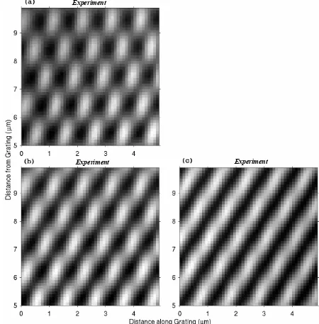
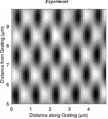
5.5 Results And Discussion 83
5.5.1 Constant Gap Evanescent Field Imaging Of A Fibre Grating 83
5.5.1.1 On-Resonance vs Off-Resonance 83
5.5.1.2 An Estimation Of ∆n From The Off-Resonance Ratio Of Intensities 87 5.5.1.3 One-Dimensional Resonant Line Scans 87 5.5.1.4 The Effect Of Moving Far From Resonance 91 5.5.1.5 Visual Identification Of Topographically Induced Artifacts 92 5.5.1.6 Large Scale Two-Dimensional Images 95
5.5.2 Decay Constant Measurements 97
5.6 Chapter Summary 99
5.7 References 101
6. Comparative Study Of The Evanescent Fields Of Two Holographically Side-Written Multi-Mode Fibre Bragg Gratings
6.1 Chapter Introduction 103
6.2 Preparation Of The Samples 103
6.3 Experimental Procedure 104
6.4 Results And Discussion 105
6.4.1 Constant Gap Evanescent Field Imaging 107
6.4.1.1 Determination Of The Average Effective Refractive Index 107 6.4.1.2 One-Dimensional Resonant Line Scans 107
6.4.1.3 Two-Dimensional Resonant Scans 110
6.4.1.4 Off-Resonance Scans 115
6.5 Chapter Summary 121
6.6 References 123
7. Comparative Study Of The Evanescent Fields Of Three Holographically Side-Written Single-Mode Fibre Bragg Gratings
7.1 Chapter Introduction 124
7.2 Preparation Of The Single-Mode Samples 124
7.3 Experimental Procedure 129
7.4 Results And Discussion 129
7.4.1 Constant Gap Evanescent Field Imaging 131
7.4.1.1 Fibre Grating Sample No.4: One-Dimensional Scans 131 7.4.1.2 Fibre Grating Sample No.4: Two-Dimensional Scans 137 7.4.1.3 Fibre Grating Sample No.5: One-Dimensional Scans 138
7.4.1.4 Fibre Grating Sample No.5: Two-Dimensional Scans 143 7.4.1.5 Fibre Grating Sample No.6: One-Dimensional Scans 145 7.4.1.6 Fibre Grating Sample No.6: Two-Dimensional Scans 148 7.4.2 Fibre Grating Sample No.6: Free-Space Evanescent Field Imaging 151
7.4.3 Decay Constant Measurements 152
7.5 Chapter Summary 156
7.6 References 157
8. Conclusions
8.1 General Conclusions 159
8.2 Future Work 162
8.3 References 163
Appendices
Appendix A: Publications 165
Appendix B: Operation Amplifier 166
Appendix C: PID Circuit Diagram 167
Appendix D: Technical Drawings 168
Acknowledgements
Warm thanks go to Bill, Barry, Chris and Ping, who have all helped to make this project possible. Also to my family, Laura, Ben and Doms, who have lived the whole experience every step of the way!
1. Introduction
1.1 General Introduction
In 1928, the British scientist E.H. Synge suggested a method of performing optical microscopy beyond the diffraction limit [1.1]. His idea consisted of raster scanning a sub-wavelength aperture in close proximity to a sample. Unfortunately, there was no way at that time to verify the technique experimentally due to the requirements of fine positioning, and it was soon forgotten. However in 1972, Ash and Nichols did manage to demonstrate two-dimensional, sub-wavelength imaging to a resolution of λ/20, by using microwave radiation [1.2]. It was not until the invention of the Scanning Tunneling Microscope (STM) by Binnig and Rohrer in 1982 [1.3], that the positioning techniques became available to enable sub-wavelength imaging at visible wavelengths. The Scanning Near-field Optical Microscope (SNOM) was subsequently born following its development by two groups [1.4, 1.5].
By around the end of the 1980’s, the use of a tapered optical fibre, coated in an opaque metal film except for at its apex, became the standard way of producing the required sub-wavelength aperture [1.6, 1.7]. However, a particular mode of SNOM operation that has come to be known as Photon Scanning Tunneling Microscopy (PSTM) in analogy with STM, utilizes an uncoated optical fibre probe in order to measure evanescent fields external to a sample, generated by total internal reflection (TIR) within the sample [1.8]. The method has already been
successfully employed to investigate the evanescent field properties of several types of optical wave-guide [1.9, 1.10, 1.11]. This thesis will expand on the work by presenting a
comprehensive PSTM examination of the external evanescent fields of six separate optical fibre Bragg gratings [1.12].
A well-established method of producing a fibre Bragg grating is to expose a photosensitive optical fibre to periodic interference fringes of UV light [1.13]. This introduces a periodic modulation into the refractive index along a length of its core. Recently, the use of a
1.2 The Motivation For The Research:
1.2.1 SNOM Imaging Of Fibre Bragg Gratings
The fibre Bragg grating is currently used extensively throughout the telecommunications industry [1.16, 1.17]. The device can be manufactured with well controlled reflection and transmission characteristics, which are presently examined in several ways. The most general of these is a measurement of the grating’s reflection and transmission spectra, to gain
information about such things as the Bragg wavelength, bandwidth and scattering from the grating region [1.18]. The use of simulation is an excellent way of gaining more information from these spectra, for example it is possible to identify phase-mask stitching errors from a spectrum’s bandwidth and associated noise [1.19]. Alternative techniques exist for assessing the refractive index profile of a grating, such as the ‘side scatter’ method [1.20], or the application of a ‘heat scan’ for probing the chirp of a grating [1.21, 1.22]. Diffraction limited photographic imaging of the grating fringes of fibre gratings has also been achieved [1.23]. However, none of the above methods can give localized, sub-wavelength information about either the actual electric field distribution within a fibre grating, or its refractive index profile, and therefore this valuable information can be lost. Indeed, Transmission Electron Microscopy (TEM) has been utilized in order to identify regions of densification caused by UV irradiation [1.24]. This too has its limitations in the respect that it does not give any information about the way that the light is propagating through the grating. Clearly, the electric field intensity and the physical structure of a fibre grating are intimately linked, and therefore high-resolution
information on both could be extremely useful.
In 1993, D. P. Tsai et al achieved the sub-wavelength imaging of the intensity modulated by a fibre grating at the interface between its core and cladding by utilizing Aperture Photon
new technique will be complementary to existing fibre grating characterization procedures, in addition to offering new insight into the structure of gratings.
1.2.2 SNOM Imaging Of Phase-Mask Diffraction Patterns
The pattern formed close to a phase diffraction grating was first observed by Talbot [1.26] in 1836. The Talbot diffraction pattern is interesting because under certain conditions, it replicates the pattern of the original grating at periodic distances from its surface, subject to diffraction limits. Rayleigh first deduced the repeat length of the pattern, known as the Talbot length, in 1881 [1.27]. The actual electric field distribution in the pattern can be calculated using finite-element models [1.28], scalar Fresnel-Kirchoff diffraction theory [1.29] or with analytical functions [1.30] to provide extremely detailed information about its amplitude and phase. Techniques involving exposure of photoresists [1.30] have been used to try to characterize the field distributions experimentally but up to now, comprehensive experimental measurements of these patterns have not been carried out. As mentioned above, the phase grating diffraction patterns are utilized to fabricate fibre Bragg gratings, and therefore a thorough analysis of these free-space patterns under real experimental conditions, is useful to engineers working in the industry. The measurements would also serve as a confirmation of theory, which up to now has been the only reliable method of visualizing these sometimes complex patterns.
1.3 Introduction To The Main Sections Of The Thesis:
1.3.1 Chapter 2: Theory
This chapter contains background theoretical issues not covered elsewhere in the thesis. It discusses matters pertaining to the mechanical operation of the SNOM, and its ability to measure optical fields. Considerations are also made relating to fibre Bragg gratings.
1.3.2 Chapter 3: Construction Of The Scanning Near-field Optical Microscope
To enable the acquisition of the data for this thesis, a Scanning Near-field Optical Microscope was designed and constructed, as part of the overall project. This chapter describes the
operation of the complete SNOM system and introduces some data acquired early on in the project, in order to demonstrate its performance. The chapter goes on to explain how the SNOM’s fibre probes were produced, and how the electronics were implemented in order to control the position of each probe, enabling the acquisition of the topographical and optical data.
1.3.3 Chapter 4: Free-Space Imaging Of Phase-Mask Diffraction Patterns
During this chapter, the measured free-space phase-mask diffraction patterns along with many associated simulations, both analytical and numerical are shown. A variety of experimental situations are given against the background of a discussion relating to fibre Bragg grating manufacture by phase-mask. In addition, an original mathematical expression, derived during the course of this project will be introduced. It relates to the Talbot Length of repeating diffraction patterns, and is most useful where few diffracting orders are present, as in the case of fibre grating manufacture at telecommunication wavelengths. The new expression is confirmed by experiment in every instance.
1.3.4 Chapters 5-7: Evanescent Field Imaging Of Fibre Bragg Gratings
analysis of data acquired early in the project from a single fibre grating is expanded into a comparative study of other gratings. Finally, a wider discussion ensues in order to coalesce all of the results in this thesis, including some of those from Chapter 4.
1.3.5 Chapter 8: Conclusions
This chapter presents the conclusions of the thesis, and offers suggestions for future work.
1.4 Chapter Summary
After a brief historical perspective on Scanning Near-field Optical Microscopy, the motivation behind the research presented in this thesis was explained. Finally, an outline has been given relating to the contents of the remainder of this thesis.
1.5 References
[1.1] E.H. Synge, Phil. Mag., 6, 356 (1928)
[1.2] E.A. Ash, G. Nichols, Nature, 237, 510 (1972)
[1.3] G.Binnig, H. Rohrer, Helv. Phys. Acta, 55, 726 (1982)
[1.4] D.W. Pohl, W. Denk, M. Lanz, Applied Physics Letters, 44, 651 (1984)
[1.5] A. Harootunian, E. Betzig, M. Isaacson, A. Lewis, E. Kratschmer, Applied Physics Letters, 49, 674 (1986)
[1.6] H. Heinzelmann, D.W. Pohl, Appl. Phys. A, 59, 89 (1994) [1.7] E. Betzig, J. Trautman, Science, 257, 189 (1992)
[1.8] R.C. Reddick, R.J. Warmack, D.W. Chilcott, S.L. Sharp, T.L. Ferrell, Rev. Sci. Instrum., 61 (12), 3669 (1990)
[1.9] A.G. Choo, M.H. Chudgar, H.E. Jackson, G.N. De Brabander, M. Kumar, J.T. Boyd, Ultramicroscopy, 57, 124 (1995)
[1.10] S. Bourzeix, J.M. Moison, F. Mignard, F. Barthe, Applied Physics Letters, 73 (8), 1035 (1998)
[1.11] D.P. Tsai, H.E. Jackson, R.C. Reddick, S.H. Sharp, R.J. Warmack, Applied Physics Letters, 56 (16), 1515 (1990)
[1.12] D. Weidman, Laser Focus World, 99, March (1999)
[1.14] K.O. Hill, B.Malo, F. Bilodeau, D.C. Johnson, J. Albert, Applied Physics Letters 62, 1035 (1993)
[1.15] E. Wolf, J.T. Foley, Optics Letters, 23 (1), 16 (1998)
[1.16] K.O. Hill, Y. Fujii, D.C. Johnson, B.S. Kawasaki, Applied Physics Letters, 32 (10), 647 (1978)
[1.17] P.E. Dyer, R.J. Farley, R. Giedl, K.C. Byron, D.Reid, Electronics Letters, 30 (11), 860 (1994)
[1.18] R. Kashyap, Fiber Bragg Gratings, Academic Press, London, 409 (1999) [1.19] F. Ouellette, P.A. Krug, R. Pasman, Optical Fiber Technol., 2, 281 (1996) [1.20] P. Krug, R. Stolte, R. Ulrich, Opt. Lett., 20 (17), 1767 (1995)
[1.21] W. Margulis, I.C.S. Carvalho, P.M.P. Govea, Opt. Lett., 18 (12), 1016 (1998) [1.22] S. Sandgren, B. Sahlgren, A. Asseh, W. Margulis, F. Laurell, R. Stubbe, A. Lidgard, Electron. Lett., 31, 665 (1995)
[1.23] B. Malo, D.C. Johnson, F. Bilodeau, J. Albert, K.O. Hill, Optics Letters, 18 (15), 1277 (1993)
[1.24] P.Cordier, S. Dupont, M. Douay, G. Martinelli, P. Bernage, P. Niay, J.F. Bayon, L. Dong, Appl. Phys. Lett., 70 (10), 1204 (1997)
[1.25] D. P. Tsai, J. Kovacs, M. Moskovits, Ultramicroscopy, 57, 130 (1995) [1.26] H. Talbot, Phil. Mag. 9, 401 (1836)
[1.27] Lord Rayleigh, Phil. Mag. 11, 196 (1881)
[1.28] G. Wojcik, J. Mould, Jr., R. Ferguson, R. Martino, K. K. Low, SPIE Proceedings 2197: Optical/Laser Microlithography VII, 455 (1994)
[1.29] J.D. Prohaska, E. Snitzer, J. Winthrop, Applied Optics, 33 (18), 3896 (1994) [1.30] P.E. Dyer, R.J. Farley, R. Giedl, Optics Communications 115, 327 (1995)
[1.31] B. Hecht, H. Bielefeldt, Y.Inouye, D.W.Pohl, L.Novotny, J. Appl. Phys, 81 (6), 2492 (1997)
2. Theory
2.1 Chapter Introduction
The background theory associated with the research carried out for this PhD project, is given in this chapter. Firstly, a discussion relating to SNOM optical measurements is followed by a description of the mechanisms that allow SNOM probes to be held close to a sample surface, enabling both evanescent components of light to be detected, and topographical measurements to be performed. Uniform fibre Bragg grating theory is also introduced, along with some details associated with the UV-photosensitivity of doped silica.
Additional theory that was developed actually during the course of this project will not be shown in this chapter, but will appear later in the thesis within the context of associated data. This consists of a new expression for the ‘Talbot length’, which will be introduced in Chapter 4, and some aspects relating to Photon Scanning Tunneling Microscopy (PSTM) measurements of fibre Bragg gratings, which will be detailed in Chapter 5.
2.2 SNOM Acquisition Of Optical Data
2.2.1 Imaging Beyond The Diffraction Limit
The difficulty associated with achieving sub-wavelength resolution with conventional optics has been known for well over a century. It was expressed in terms of diffraction theory by Abbe in 1873 [2.1], and was later reformulated by Lord Rayleigh [2.2] in the following concise form
) sin( 2
22 . 1
θ λ n
r≥ . (2.1)
assuming propagating waves. By utilizing SNOM, the detection of non-radiating (evanescent) fields can be realised, allowing this diffraction limit to be circumvented.
2.2.2 The Angular Spectrum Of The Object Field
In order to demonstrate that the evanescent field contains information about the highest spatial frequencies of an object, therefore holding the key to increased resolution, an angular spectrum analysis offers a lucid description [2.3]:
A two-dimensional limited object, described by its transmittance or reflectance f(x,y,0), may be expressed in the form of a two-dimensional Fourier integral
∫ ∫
+∞ ∞ − + −= f x y i ux vy dxdy
v u
F0( , ) ( , ,0)exp[ 2π( )] (2.2)
where u, are the spatial frequencies of the object. The object bounding means that v F0(u,v)
contains all possible frequencies, from zero to infinity. If a plane wave with uniform amplitude impinges on the limited object, to a first approximation, the field immediately beyond the object can be written
U(x,y,0)= f(x,y,0). (2.3) The two-dimensional Fourier transform
∫ ∫
+∞∞ −
+
= F u v i ux vy dudv
y x
U( , ,0) 0( , )exp[2π( )] (2.4)
therefore allows the object field to be regarded as the superposition of a collection of exponential functions where the terms exp[i2π(ux+vy)] correspond to elementary plane waves with direction cosines
α =λu β =λv γ =[1−λ2(u2 +v2)]1/2 (2.5) where λ is the wavelength of the illuminating light. Equation (2.2) can therefore be regarded as the angular spectrum of the object field U(x,y,0). Substituting Equations (2.3) and (2.5) into (2.2), and using k= 2π /λ gives
∫ ∫
+∞ ∞ − + −= U x y ik x y dxdy
k k
Since no restrictions have been put on the location of the observation plane, the distance from
the object z can be chosen to be much smaller than the wavelength. Equation (2.4) then gives
∫ ∫
+∞∞ −
+
= α π β π α β α β
π F k k z ik x y d d
k z y x
U ( /2 , /2 , )exp[ ( )]
4 ) , , ( 2 2
. (2.7)
Finally, by utilizing Equations (2.6) and (2.7) in conjunction with the Helmholtz equation [2.4], the angular spectrum at a distance z from the object plane can be expressed as [2.2]
( /2 , /2 , ) ( /2 , /2 )exp[ (1 2 2)1/2 ]
0 k k ik z
F z k k
F α π β π = α π β π −α −β (2.8)
where F0(αk/2π,βk/2π) is the angular spectrum of the field in the object plane (z=0). Equation (2.8) shows that the ability for plane wave components to propagate, depends on their direction cosines. For example, if
α2+β2 <1 (2.9) then the plane waves are able to propagate from the object to the detector, but if
α2+β2 >1 (2.10) then the waves are strongly attenuated in the z-direction. The plane waves in the latter case correspond to evanescent waves, which can be expressed in the following manner
F(αk/2π,βk/2π,z)=F0(αk/2π,βk/2π)exp[−k(α2 +β2 −1)1/2z] (2.11) where the direction cosines depend on object structure from Equations (2.2) and (2.5). The Rayleigh criterion can be deduced from Equations (2.5) and (2.9) by introducing a one-dimensional object where v = 0 [2.3]. From this, the largest propagating spatial frequency would be given by
u=k/2π (2.12) and therefore the highest spatial frequency in the detected far-field equates to
u'= 2u=k/π (2.13) which is a result that is comparable to that given in Equation (2.1).
Equation (2.11) is formally analogous to
( /2 , /2 , ) ( /2 , /2 )exp{ [( )2 ( )2 1]1/2 }
0 k k k n n z
F z k k
F α π β π = α π β π − α + β − (2.14)
which describes the generation of evanescent waves at a total internal reflection (TIR) interface, where αand βare the two direction cosines of the incident wave and n is the
thesis as Equation (5.2), where the generation of TIR evanescent fields is discussed within the context of PSTM.
The relationship between high spatial frequencies and the generation of non-propagating evanescent fields could also have been arrived at by solving Maxwell’s equations [2.5, 2.6], or by utilizing the Heisenberg uncertainty principle [2.7]. However, the angular spectrum model is a particularly useful description, because it makes clear the role of the evanescent components. It also gives an insight into how the evanescent fields relate to detection by a SNOM probe, situated at a particular distance z from a sample.
2.2.3 SNOM Detection Of Components Of The Object Field
The SNOM probes used during this project are described in Chapter 3 of this thesis. However, they basically take two forms: an optical fibre tapered at one end down to a ~50nm diameter [2.8], and a tapered optical fibre coated in aluminium to leave a tiny aperture at its apex [2.9]. The detection of non-radiating fields by the former probe, has been described in various ways. A simple method assumes that the tip of the probe behaves like a dipole [2.10] which, when placed within the proximity of a non-radiating field, is excited and generates an
electromagnetic field consisting of both propagating and non-propagating components [2.11]. The propagating components are subsequently guided along the probe’s fibre to be recorded by
a remote detector. In this case, each evanescent field component E(x,y,z) induces on the tip
an electric dipole AE(x,y,z), and the subsequent detected intensity is given by [2.12]
]} 3 cos 2 cos 18 16 [ | ) , , ( | ] 3 cos cos 15 16 ][ | ) , , ( | | ) , , ( {[| | | 96 ) , , ( 2 2 2 2 3 4 δ δ δ δ ω + − + − − + = z y x E z y x E z y x E A c z y x I z y x d (2.15)
where ωis the frequency of the incident light, c is the speed of light in a vacuum, δ is the collection angle of the tip, i.e. the half angle of its taper and A is the polarizability of the tip. If the apex of the optical fibre probe is considered to be a small sphere of radius R and dielectric constant εtip, then the polarizability can be written [2.13]
3 2 1 R A tip tip + − = ε ε
Many other theoretical approaches have been taken to model the detection of light by SNOM probes. In a similar manner to the above description, some have assumed that the detected signal is proportional to the square modulus of the electric field at the tip position [2.14, 2.15]. Another point of view has been to describe the tip as a point-like scatterer, which scatters the evanescent near-field towards a far-field detector [2.16, 2.17].
The discussion above has been principally based upon the detection of non-radiating fields with an uncoated SNOM probe. This can be related to the data shown in Chapters 5-7 of this thesis, which carries out this function. However, in Chapter 4, an aluminized SNOM tip positioned some distance away from an illuminated sample is used. The measurements include only radiating components because the tip is out of the range of the quickly decaying evanescent fields. However, by the reciprocity theorem [2.18, 2.19], both evanescent and radiating fields incident on a SNOM tip will be converted partly into propagating components that can be measured by a detector [2.20]. The reason for aluminizing the tip here, was in order to prevent light incident on the probe from passing into the cladding of the fibre along its tapered region. This would have resulted in an increase in the sampled area of measurement, and consequently a reduction in resolution.
2.3 SNOM Probe Oscillation And Interaction With Sample
The positioning of a SNOM tip close to a sample is necessary in order to detect the bound evanescent fields. It was achieved during this project by attaching the probe to an oscillating quartz tuning-fork, allowing for a slight tip overhang. A monitoring of the damping effect on the tip by surface shear forces enabled the probe’s height to be fixed relative to the sample [2.25]. The exact nature of the shear force is still unclear but is thought to be a combination of various forces such as electrostatic, capillary and van der Waals [2.26, 2.27]. What is clear however, is that the sample surface water layer can contribute to damping, and therefore the overall effect of the shear force can vary over time [2.28]. This effect was confirmed during the course of this PhD project.
The vibrating probe can be modeled as a classical driven harmonic oscillator [2.29] with an equation of motion given by [2.30]
2 sin( ) 2 t F kx dt dx dt x d
m +γ + = a ω (2.17)
where the terms on the left are the inertial, damping and restoring forces respectively, and the term on the right is the driving force. The quantity mrepresents the effective mass, γ is the damping coefficient, k is the spring constant, Fa is the driving force amplitude applied to the
tuning-fork, ω is the driving frequency and the vibration amplitude at the tip of the probe is given by
x=Xsin(ωt+ϕ) (2.18) where ϕ is the phase shift between the drive and the tip’s response. The response amplitude is calculated by substitution of derivatives of Equation (2.18) into Equation (2.17), to give [2.29]
2 0 2 2 0 2 1 / ) ( + − = ω ω ω ω ω Q k F X a (2.19)
where ω0 is the undamped natural frequency, the quality factor is given by
ω ω ∆ = 0
and ∆ω is the FWHM of the resonance. Examination of Equation (2.19) shows that a decrease in tip amplitude X , as a result of its interaction with sample shear forces, can be either due to a decrease in the quality factor Q corresponding to an increase in γ , or a shift in resonant
frequency ω0, resulting from a force in the direction of the probe dither motion [2.29].
As will be demonstrated in Chapter 3 of this thesis, the theoretical consequences of tip damping as discussed above, will be confirmed by experiment.
2.4 Uniform Fibre Bragg Gratings
A PSTM investigation of the evanescent fields of several fibre Bragg gratings is shown throughout Chapters 5-7 of this thesis. All of the fibre gratings used were created to have a uniform period of refractive index variation along their length, and are therefore known as ‘uniform gratings’. This section will give an introduction to uniform fibre grating theory in order to support some of the discussion and analysis that follows later in this thesis. However, it will not cover aspects relating to a grating’s evanescent field, as this topic will be evaluated in Chapter 5.
Fibre Bragg gratings are formed by exposing an optical fibre with a photosensitive core to periodic fringes of UV light [2.42]. The consequence of this is that a perturbation in the
effective refractive index ne ensues, along the affected length of the core. With the z-direction
along the core’s axis, the induced perturbation can be described by [2.33]
Λ +
= n z z
z
ne e
π ν
δ
δ ( ) ( ) 1 cos 2 (2.21)
where δne is the average index change along the length of the grating, ν is the fringe visibility of the index variation and Λ is the period of the grating. The fibre grating performs like a simple optical diffraction grating and therefore light traveling along its fibre and becoming incident on the grating at angle θ1, will be diffracted at angle θ2 according to the
grating equation [2.43]
Λ +
= θ λ
θ n m
where m defines the diffraction order. The mode propagation constant, or axial component of the wave vector, is given by [2.33]
β =nksinθ =nek (2.23) where ne is the average effective refractive index and
λ
π 2 =
k . (2.24)
Combining Equations (2.22) and (2.23) gives
Λ +
=β π
β2 1 m2 . (2.25)
For first order diffraction, which dominates in fibre Bragg gratings, m=−1 describes a
reflection condition [2.33]. Additionally, negative β values describe modes that propagate in the reflection direction. Given that this is the case, Equations (2.23) and (2.25) can be utilized to give
Λ − =
−kne,2 kne,1 2π (2.26)
which, when combined with Equation (2.24) gives
λ=(ne,1 +ne,2)Λ. (2.27) The resonant wavelength for coupling of a forward propagating mode to a backward
propagating mode is given when ne,1 =ne,2 leading finally to the condition for Bragg reflection λB =2neΛ (2.28)
where λB is the Bragg wavelength.
The periodically varying refractive index along the length of a fibre grating provides multiple reflections to incident light. The total macroscopic response of the grating can therefore be illustrated more formally by coupled-mode theory, which describes the coupling of counter-propagating guided waves [2.31, 2.44]. Given that A(z) and B(z) are the amplitudes of the forward and backward propagating waves respectively, the total device response can be described by
E z A z e i 0z B z ei 0z
) ( )
( )
where β0 =π /Λ, and is equivalent to the propagation constant given in Equation (2.23), at the Bragg wavelength. Significantly, the use of coupled-mode theory to describe single-mode, uniform fibre Bragg gratings has enabled the derivation of an expression for the reflection bandwidth, which is given by [2.31, 2.33]
2
1
+ = ∆ L n n n e e e δ λ δ λ λ (2.30)
where L is the overall length of the fibre grating and ∆λ is the width between the first two zero reflection regions, either side of the maximum reflectivity. The expression is utilized in this thesis to estimate values of induced refractive index.
2.5 UV Photosensitivity Mechanisms In Doped Silica Optical Fibres
Photosensitivity utilized for grating writing in optical fibres is predominantly associated with oxygen deficiencies in the chemical structure of a fibre [2.34]. For example, in a germanium-doped silica fibre core, the photosensitivity has been correlated with the concentration of GeO defects [2.35, 2.36]. It is a consequence of the atom immediately adjacent to a germanium atom being either silicon or another germanium, resulting in a bond with a characteristic 240nm absorption peak [2.37]. When illuminated with UV light, the bond breaks creating a GeE’ centre. The breaking of the bond, and thus the liberation of an electron causes a reconfiguration of the shape of the molecule, possibly also changing the density of the material [2.38]. The addition of boron to this type of fibre core has the effect of reducing the background refractive index. This allows a higher concentration of the index-increasing germania, resulting in greater photosensitivity, without significantly affecting the fibre’s refractive index profile. All of the Bragg grating samples examined in this thesis were germania-boron co-doped silica fibres.
~200 bar for about two weeks at room temperature, is adequate to load a fibre with 125µm diameter [2.41].
2.6 Chapter Summary
This chapter has introduced some of the background theory associated with the acquisition of data for this thesis, by explaining the main concepts of Scanning Near-field Optical Microscopy (SNOM). The chapter has also discussed theoretical issues associated with fibre Bragg gratings, which are devices associated with the majority of the work carried out during this project.
2.7 References
[2.1] E. Abbe, Archiv f. Miroskop. Anat., 9, 413 (1873) [2.2] D. Courjon, C. Bainier, Rep. Prog. Phys. 57, 989 (1994)
[2.3] D. Courjon, J.-M. Vigoureax, M. Spajer, K. Sarayeddine, S. Leblanc, Applied Optics, 29
(26), 3734 (1990)
[2.4] J.W. Goodman, Introduction to Fourier Optics, Mcgraw-Hill, London, 48-55 (1968) [2.5] H.A. Bethe, Phys. Rev., 66, 163 (1944)
[2.6] C.J. Bouwkamp, Philips Res. Rep., 5, 401 (1950)
[2.7] J.M. Vigoureux, D. Courjon, Applied Optics, 31 (16), 3170 (1992)
[2.8] G.A. Valaskovic, M. Holton, G.H. Morrison, Applied Optics, 34 (7), 1215 (1995) [2.9] C.W. Hollars, R.C. Dunn, Review of Scientific Instruments, 69 (4), 1747 (1998) [2.10] D. Van Labeke, D. Barchiesi, J. Opt. Soc. Am. A, 9, 732 (1992)
[2.11] E. Wolf, M. Nieto-Vesperinas, J. Opt. Soc. Am., 2, 886 (1985)
[2.12] D. Van Labeke, D.Barchiesi, Near Field Optics, Kluwer Academic, 157-178 (1993) [2.13] B. Labani, C. Girard, D. Courjon, D. Van Lebeke, J. Opt. Soc. Amer. A, 7, 936 (1990) [2.14] C. Girard, A. Dereux, Rep. Prog. Phys., 59, 657 (1996)
[2.15] J.J. Greffet, R. Carminati, Prog. Surf. Sci., 56, 133 (1997) [2.16] C. Girard, D. Courjon, Phys. Rev. B, 42, 9340 (1990)
[2.17] D. Van Labeke, D. Barchiesi, J. Opt. Soc. Am. A, 10, 2193 (1993)
[2.18] L. Landau, E. Lifshitz, L. Pitaevskii, Electrodynamics of Continuous Media, Pergamon, Oxford (1984)
[2.20] A. Dereux, Ch. Girard, J-C. Weeber, J. Chem. Phys., 112, 7775 (2000) [2.21] C.J. Bouwkamp, Philips Res. Rep., 5, 321 (1950)
[2.22] B. Hecht, B. Sick, U.P. Wild, V. Deckert, R. Zenobi, O.J.F. Martin, D.W. Pohl, Journal Of Chemical Physics, 112 (18), 7761 (2000)
[2.23] D.V. Labeke, D. Barchiesi, F. Baida, J. Opt. Soc. Am. A, 12, 695 (1995) [2.24] A Roberts, J. Appl. Phys., 70 (8), 4045 (1991)
[2.25] K. Karrai, R.D. Grober, Applied Physics Letters, 66 (14), 1842 (1995) [2.26] E. Betzig, P.L. Finn, J.S. Weiner, Applied Physics Letters, 60, 2484 (1992)
[2.27] R. Toledo-Crow, P.C Yang, Y. Chen, M. Vaez-Iravani, Applied Physics Letters, 60,
2957 (1992)
[2.28] S. Davy, M. Spajer, D. Courjon, Applied Physics Letters, 73 (18), 2594 (1998) [2.29] F.F. Froehlich, T.D. Milster, Applied Physics Letters, 70 (12), 1500 (1997)
[2.30] D. Sarid, Scanning Force Microscopy, Oxford University Press, New York (1991) [2.31] R. Kashyap, Fiber Bragg Gratings, Academic Press, London, 142-145 (1999)
[2.32] E. Kreyszig, Advanced Engineering Mathematics, 5th Edition, Wiley, New York, 345 (1992)
[2.33] T. Erdogan, Journal of Lightwave Technology, 15 (8), 1277 (1997)
[2.34] I. Bennion, J.A.R. Williams, L. Zhang, K. Sugden, N.J. Doran, Optical and Quantum Electronics, 28, 93 (1996)
[2.35] D.L. Williams, S.T. Davey, R. Kashyap, J.R. Armitage, B.J. Ainslie, SPIE, 1513, 158
(1991)
[2.36] B. Poumellec, P. Niay, M. Douay, J.F. Bayon, J. Phys. D, Appl. Phys., 29, 1842 (1996) [2.37] A.J. Cohen, H.L. Smith, J. Phys. Chem., 7, 301 (1958)
[2.38] R. Kashyap, Fiber Bragg Gratings, Academic Press, London, 16-29 (1999)
[2.39] F. Bhakti, J. Larrey, P. Sansonetti, B. Poumellec, Bragg Gratings, Photosensitivity and Poling in Glass Fibers and Waveguides: Fundamentals and Applications, OSA Technical Series, paper BSuD2, 17, 55 (1997)
[2.40] R. Kashyap, Fiber Bragg Gratings, Academic Press, London, 29-35 (1999)
[2.41] P. Lemaire, R.M. Atkins, V. Mizrahi, W.A. Reed, Electron. Letts., 29 (13), 1191 (1993) [2.42] G. Meltz, W.W. Morey, W.H. Glenn, Optics Letters, 14, 823 (1989)
3. Construction Of The Scanning Near-field
Optical Microscope (SNOM)
3.1 Chapter Introduction
The Scanning Near-field Optical Microscope (SNOM) used to obtain the data for this PhD thesis was designed and built as part of the overall project. Although the apparatus evolved over a period of several months and included many stages of improvement, this chapter
describes only the final set-up of equipment. A characterization of the operational performance of the SNOM is ongoing throughout the chapter. The chapter begins with an overview of the operation of the complete SNOM system, followed by a description of its individual
components. Finally, some corresponding experimental details are given, along with relevant data.
3.2 An Outline Of The SNOM’s Operation And Its Components
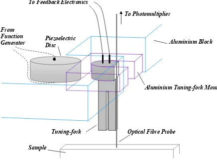
The design of the SNOM, which was based on an idea by K. Karrai and R. D. Grober [3.1], consisted of a high Q-factor quartz tuning-fork that was used as a mount upon which a tapered optical fibre probe with a 50-100nm tip [3.2] was positioned and glued with a slight tip
overhang, as seen in Figure 3.1. The tuning-fork/probe system was forced to oscillate at its resonant frequency by a nearby piezoelectric disc, with the result that the probe acquired a dithering motion [3.3]. With the overall dither assembly mounted such that its movement in three-dimensions could be controlled by a piezoelectric translation stage, the fibre probe could be made to approach a sample, whereupon its dither would be dampened by surface forces close to the sample [3.4, 3.5]. Since the amplitude of dither, and therefore the tuning-fork induced voltage, was dependent upon the distance between the tip and sample, it could be monitored by means of feed-back electronics, in order to control the probe’s height [3.6, 3.7]. By fixing the height of the tip relative to the sample, computer controlled raster scanning over its surface enabled acquisition of data relating to sample topography. In addition, connection of a photomultiplier tube to the opposite end of the probe’s fibre enabled simultaneous
Figure 3.1: The Dither Assembly and sample. The optical fibre tip was super-glued to the quartz tuning-fork, which itself was super-glued to the aluminium tuning-fork mount. Likewise, the tuning-fork mount was attached with super-glue to the piezoelectric disc, whilst being allowed to oscillate freely within the cut away section of the aluminium block. The piezoelectric disc was fixed within the block from below. The aluminium block was bolted to an invar cantilever, which was mounted upon an xyz piezoelectric stage. See Figure 3.2 and subsequent text for more details.
moving the tip away from the sample, optical field intensity in regions of ‘free-space’ could be recorded at various heights above the sample [3.9, 3.10], corresponding to positions out of the range of the sample’s surface forces.
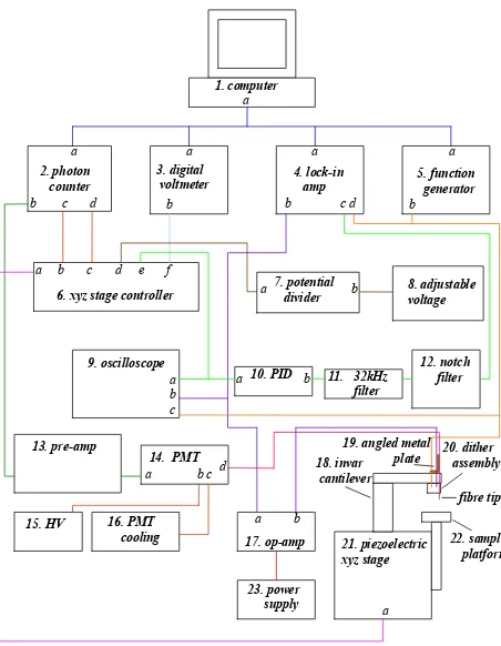
Figure 3.2 shows a schematic of the complete set-up of equipment that combine to make the SNOM. All the items shown are explained in the text immediately following the figure.
Piezoelectric Disc
Optical Fibre Probe Tuning-fork
Aluminium Tuning-fork Mount Aluminium Block
Sample
To Photomultiplier To Feedback Electronics
From Function Generator
Figure 3.2: Layout and connection of the equipment that combine to make up the SNOM. Inputs and outputs represented by letters, are explained in the following text.
1. computer
2. photon counter
3. digital
voltmeter 4. lock-in amp 5. function generator
6. xyz stage controller 7. potential divider
11. 32kHz filter
8. adjustable voltage
9. oscilloscope
10. PID 12. notch filter
13. pre-amp
15. HV 16. PMT
cooling 17. op-amp
23. power supply 21. piezoelectric xyz stage 18. invar cantilever 20. dither assembly 22. sample platform 14. PMT
b c d b b c d
a a
a
a a
b
a b c d e f
a b
a b c
a b
a b c d
a a b
fibre tip 19. angled metal
Description of the equipment shown in Figure 3.2.
1. Computer; Dell P60. Belkin F1D090E data switch to additional monitor, keyboard and mouse situated in adjoining office. Various computer programs to operate adjoining equipment were written in ‘C’ and ‘C++’. Output a: GPIB port.
2. Photon Counter; Stanford Research Systems SR400. Input a: IEEE interface. Input b: photon count from PMT, (dark count 20-30 c/s). Output c: port 1, ±10V to stage
controller y input (sum). Output d: port 2, ±10V to stage controller x input (sum). 3. Digital Voltmeter; Keithley 196 System, serial no. 371567. Input a: IEEE interface.
Input b: 0-10V signal from stage controller, equating to ~(0-19.7)µm z-direction movement. This instrument monitored height of the SNOM tip.
4. Lock-in Amp; Stanford Research Systems SR530, serial no. 06776. Input a: IEEE interface. Input b: signal from tuning-fork (A input). Output c: Y component of
tuning-fork signal relative to reference signal (±10V). Input d: reference signal from function generator.
5. Function Generator; Stanford Research Systems DS335, 3.1MHz, serial no. 26921. Input a: IEEE interface. Output b: signal equating to resonant frequency of tuning-fork/tip system, 1V p-p sine wave.
6. XYZ stage controller; Melles Griot piezoelectric controller with feed-back, serial no. 500265. Terminal a: xyz drive outputs 0-75V and xyz strain-gauge feed-back return. Input b: y sum (+). Input c: x sum (+). Input d: z sum (+). Input e, z diff (-). Output f: z height information.
7. Potential Divider; output a potential equates to 9.1% of input b potential. 8. Adjustable Voltage; Thurlby Thandar Instruments, TSX 3510P. Manually operated z
height fine positioning of tip.
9. Oscilloscope; Hitachi V-525, 50MHz. Input a: channel 2. Input b: channel 1. Input c: external trigger.
10.PID unit; built at Southampton university physics dept, circuit diagram shown in
Appendix C. Input = b, output = a. The ‘D’ element was not used during the project. 11.32 kHz filter; used to reject noise from lock-in amp.
12.Notch filter; used to reject 50Hz noise.
14.Photomultiplier; Burle Industries Inc. C31034A, serial no. V23133. GaAs
photocathode. Peltier cooled to -30 degrees Celsius. Quantum efficiency 20-30%. Anode = a, cathode = b, input c: cooling power-supply, input d: optical fibre from SNOM tip.
15.High Voltage; Brandenburg photomultiplier power supply. Fixed at 1500V.
16.PMT cooling power supply; Products For Research Inc. TE-104RF, serial no. 17363-90. 17.Op-amp; In order to achieve a measurable tuning-fork signal, a simple integrated circuit
amplifier was mounted close to the ‘dither assembly’. Input = b, output = a. Additional details and a circuit diagram are shown in Appendix B.
18.Invar cantilever; consisting of two lengths, horizontal and vertical. Designed and built during project. Technical drawing shown in Appendix D.1.
19.Angled metal plate; used to support the optical fibre, by means of two small magnets. 20.Dither assembly; shown in greater detail in Figure 3.1. Also shown attached to invar
cantilever in drawing Appendix D.4. Assembly consists of an RS Components quartz tuning-fork with prongs 4mm in length and resonant frequency 32.768kHz, its cap removed and its head filed to produce a flat surface (see Figure 3.1); aluminium tuning-fork mount 6x6x2mm; piezoelectric disc 4mm diameter; aluminium block 25x15x6mm. 21.Piezoelectric xyz stage; Melles Griot, serial no. 500155. Output a: communication link
with controller. A drawing, and performance specification are shown in Appendix D.3. 22.Sample platform; Height adjustable, designed and built as part of this project.
Adjustable upright support: aluminium. Horizontal platform: invar. Diagram shown in
Appendix D.2.
23.Power supply; Instek PC-3030. 15V supply for op-amp.
3.3 Optical Fibre Probe Preparation And Attachment
The optical fibre used to create all of the SNOM probes used during the course of this project has its details shown in Table 3.1. The process to create a tip was fairly uniform throughout the whole project. Firstly, a ~2m length of fibre was removed from its drum whereupon it had a ~1cm length of its plastic coating stripped with either acetone or dichloromethane, towards one of its ends. After cleaning the stripped area with methanol and lens tissue, the fibre was
Serial Number YD148-01
Coating Diameter 210 µm
Cladding Diameter 125µm
Single-mode cut-off 665nm
Table 3.1: Details of the optical fibre used to create all of the SNOM probes used during this project.
factory configured for drawing optical fibres. The Puller’s 10W CO2 laser being incident on the
fibre, heated the stripped section allowing it to be drawn and separated into two tips. Comprehensive details of the Sutter Puller’s operation can be found in its manual [3.11]. However, there are five user-adjustable parameters that will be summarized here.
(i) HEAT (Range 0-999). This specifies the output power of the laser, and consequently the amount of energy supplied to the glass.
(ii) FILAMENT (Range 0-15). This specifies the rate at which the laser is scanned from side to side, and the length of scan. This function was not used during the project, and therefore the incident laser beam’s position remained fixed.
(iii) VELOCITY (Range 0-255). With the fibre initially clamped under tension, the heat from the laser causes the clamping carriage to move as the glass melts. The
‘velocity’ parameter determines the speed at which the carriage should be moving when a ‘hard-pull’ is executed to separate the fibre. The velocity is dependent on viscosity, which in turn is dependent on the temperature of the glass.
(iv) DELAY (Range 0-255). This parameter controls the timing of the start of the ‘hard-pull’ mentioned above, relative to the deactivation of the laser. If DELAY < 128, then the ‘hard-pull’ is activated and HEAT turns off (128-DELAY)ms later. If DELAY >128, then the HEAT is turned off, and the ‘hard-pull’ is activated (DELAY-128)ms later.
Although there was initially some investigation into how the shape of the SNOM tip can be changed by varying the above parameters, it was decided early on in the project to adopt the
Sutter Company’s recommended settings for pulling 125µm diameter fibres [3.11]. The details are shown in Table 3.2, along with Sutter’s estimated dimensions of the resulting tip. All tips used to collect the data shown in Chapters 3-7, were created with these parameters.
HEAT 290
FILAMENT 0
VELOCITY 20
DELAY 126
PULL 150
Time to melt 0.15s
Tip diameter 50nm
Taper length 1.1mm
Table 3.2: Sutter Instrument Company recommended parameters for pulling 125µm
diameter fibre tips, and the resulting tip dimensions. These were the parameters initialized to create all of the SNOM probes used to collect the data shown in Chapters 3-7.
The procedure described thus far for creating SNOM probes is complete for the tips used to derive the evanescent field optical data shown in Chapters 5-7. However, data displayed in
Chapter 4 represents ‘free-space’ measurements of propagating light. To maximize the
The procedure to attach the prepared tip to the tuning-fork was the same for both coated and uncoated probes. Under the illumination of a Flexilux 150HL Universal Light Source and viewed through a traveling microscope, the fibre was positioned on the metal plate above the cantilever and held with a magnet, such that it was almost in contact with the tuning-fork below, yet with its tip ~2mm lower than the fork’s tines. A piece of fine wire was dipped into super-glue and subsequently ‘stroked’ along the fibre at the position of the fork. A Prior 62345 micro-manipulator was utilized to gently push the fibre against the tuning-fork until the glue had dried. A second magnet was then placed on the fibre towards the bottom of the metal plate at a distance of ~30mm from the glued region. This had the effect of stiffening the system to increase its Q-factor to a workable level.
3.4 Shear-Force Control And Topographical Data Acquisition
The details pertaining to the acquisition of topographical data will be examined here.
3.4.1 Probe Resonance And Quality-Factor
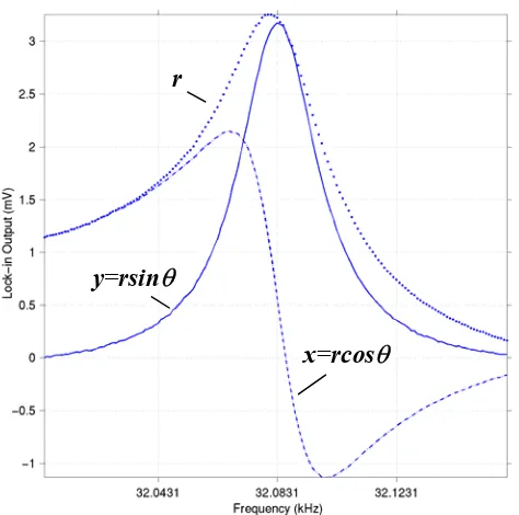
The glue holding the tip to the tuning-fork (as described above) was left to harden for about 2 hours to allow the fork/tip system’s resonant frequency and Q-factor to settle. Indeed, both qualities continued to vary marginally over the following ~24hrs, but not enough to adversely affect the SNOM’s performance in the mean time. In general, the day after a tip had been glued, an increase of about 0.1% in resonant frequency and about 5.0% in the Q-factor would be recorded compared to a measurement taken 2 hours after fixing. Figure 3.3 shows typical lock-in amplifier voltages collected by computer whilst driving a tuning-fork/uncoated-tip system through resonance. The program for retrieving this data was coded in ‘C’. The
outcomes were therefore moderately unpredictable, although a reasonable Q-factor could be obtained for all experiments.
Figure 3.3: Resonance curve of a tuning-fork/uncoated-tip system, measured 2hrs after gluing. The lock-in voltage components x (dashes), y (line) and r (dots) are shown, where r represents a value proportional to the amplitude of tip dither, x=rcosθ, y=rsinθ and θ represents the phase angle between the oscillation of the tuning-fork and the reference signal. The Q-value (resonant frequency/FWHM) of the y-component shown here is 1034. The step size per data point is 1HZ.
3.4.2 Tip-Sample Approach
During all of the work in this thesis where the tip is locked to the surface of a sample, photons were counted at each data point for at least 1 second. However, for the data shown in Figure 3.3, the settling time to 1% of the tip system for the values of y-component Q-factor and resonant frequency, equates to [3.5]
5τ = 5(2Q√3/ω0) (3.1)
= 89ms y=rsinθ
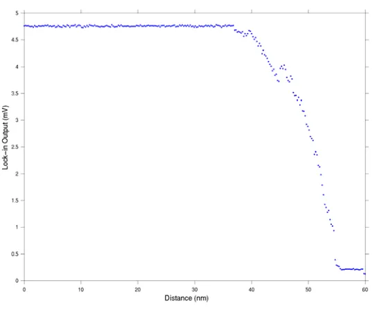
It was therefore judged convenient to use the y-component voltage of the lock-in as a basis for the feed-back loop in order to position the tip relative to a sample. Figure 3.4 shows the result of holding a tip on resonance and recording the y-component voltage of the lock-in amplifier whilst moving the tip towards the flat, silica-clad surface of a D-fibre [3.13]. The reduction in the lock-in voltage as the tip approaches the sample is mainly caused by the reduction in tip amplitude due to its interaction with surface forces, and also to a lesser degree by a slight
Figure 3.4: Surface ‘force-curve’ of an uncoated tip being lowered towards a silica sample. The y-component voltage of the lock-in amplifier is shown vs. distance of tip travel, as the tip is driven towards the sample’s surface.
determine exactly where the tip-sample contact point was as Figure 3.4 demonstrates. Over the course of this project interaction distances varied from ~20-40nm. Consequently, the
positioning of the tip at about half this height resulted in scans being performed at heights varying between ~10-20nm. The forces that are believed to give rise to SNOM probe dampening, were discussed in Chapter 2, in addition to the theory relating to a fork/probe oscillating system.
3.4.3 Probe Positioning And Initiation Of Feed-back Electronics
In order to begin surface scanning, the feed-back loop had to be initiated. Basically, with the wiring loops as shown in Figure 3.2 in place, just four operations had to be carried out to achieve this:
(1)The tip was fine-positioned by using the Thurlby voltage source such that the lock-in y -component amplitude was reduced by half.
(2)The y-component amplitude was ‘zeroed’ by pushing the lock-in amp ‘offset’ button. (3)The ‘Proportional’ element of the PID unit was initialized.
(4)The ‘Integral’ element of the PID unit was initialized.
A typical lock-in output variation of ~0.25mV/nm in response to tip movement relative to the position of the sample, can be compared to an input variation of ~0.51mV/nm for the z -height-positioning of the piezoelectric controller. However, the y-component BNC output used for the feed-back was amplified to a full scale of ±10V. Therefore the PID unit would typically receive an input of ~100mV/nm in response to tip movement relative to the sample surface. With the ‘Proportional’ dial set to zero ~(1:1 gain) and the ‘Differential’ disengaged, the ‘Integral’ function was found to have a gain of 1.931s-1 with its dial also fixed on its minimum setting.
The lowest setting on both the ‘P’ and ‘I’ sections of the unit was therefore found to be
3.4.4 Calibration Of The Piezoelectric Stage
A regular occurrence during this project was a full calibration of the xyz piezoelectric stage, with reference to the voltages used to drive the stage and record its movement. This was done by scanning a tip along a Dasaw Pty Ltd. precision diffraction grating by holding it at 45 degrees to the horizontal, and measuring its topographical period. Both x and y directions were individually checked whilst monitoring the z-displacement. An engineered glass block with its upper face inclined at the required angle was used to position the grating under the SNOM tip. The period of the grating and the angle of incline of the glass block, were checked to a high level of accuracy (±0.1%) by HeNe (632.8nm) laser diffraction and reflection respectively.
3.4.5 Stability, Repeatability And Resolution Of Acquired Topographical Data In order to investigate the stability and repeatability of any acquired height data, a
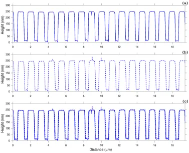
one-dimensional line-scan was performed upon a well-characterized phase diffraction grating (QPS Technology Inc. phase-mask). The computer program for achieving this was coded in ‘C’. The data can be observed in Figure 3.5(a). The grating had evenly spaced rectangular elevations 568nm apart, and therefore overall period 1136nm. The height of each elevation was calculated to be 244nm from Equation (4.1). The actual scan is over a length 19.425µm with 1025 data points, in a direction perpendicular to the grating’s rulings. Figure 3.5(b) shows a repeat run, carried out on immediate completion of the data acquisition for Figure 3.5(a). Figure 3.5(c) shows the two data sets again to enable a comparison to be made. As can be seen, there is good repeatability between the two scans, although one is laterally offset relative to the other by up to 35nm, due to thermal drift. Recorded scan lengths that exceed expected values by about 0.1% confirm the drift.
Figure 3.5: (a) A line scan across the rulings of a ‘phase-mask’ using an aluminized tip. The length of the scan is 19.425µm and has 1025 data points. The rest time at each position is 1 second, and the period of the mask is 1136nm. (b) Repeat of the scan shown in (a).
(c) Comparison of the scans shown in (a) and (b).
acquisition commenced, with its operation controlled from an external computer to assure that the acquired stability was maintained. Nevertheless, these measures did not preclude the consequence of building vibration on obtained data, as Figures 3.5(a) & (b) clearly
In order to acquire more detailed information about the resolution capability of the SNOM in its measurement of topography, a polished silica sample was scanned with the result shown in
Figure 3.7. A 7.4µm length of the sample was mapped twice, with 58nm steps in between data points. The figure shows there to be thermal drift in the +ve z-direction between the first (blue) and second (red) data sets. Of course drift in this direction has less significance than in the x &
y directions because the tip will always hold its position relative to the surface. Surface features that are about 1nm in height have been reproduced in both sets of data.
Figure 3.7: Repeat topographical measurement of a silica sample. The blue data was
acquired prior to the red data. The steps between points are 58nm, and the total length of the
scan is 7.4µm. The y-axis has been set to an arbitrary position and therefore shows relative height.
3.4.6 Probe Position Error Signal
During the acquisition of the height data shown in Figure 3.5(a), the corresponding error signal in the tip’s position relative to the sample surface was also measured. By recording the value of the y-component lock-in output at each position lastly in the data-taking sequence, a
measurement of the fluctuation in the system was gained well after its settling time. The result can be observed in Figure 3.6, where the vertical axis has been scaled such that it corresponds
to ±0.5nm tip movement. As can be seen, with a tip-sample distance of ~10nm, the stability of
the z-positioning of the probe is within ±3%.
Figure 3.6: The error in the tip position relative to the sample surface. This data was derived
simultaneously to the scan shown in Figure 3.5(a). The scan length is 19.425µm and there are 1025 data points. The rest time at each position was 1 second and the error signal was acquired last in the data acquisition sequence.
3.5 Optical Data Acquisition
The aspects relating to the collection of SNOM optical data will be presented in this section. However, theoretical details relating to the tip’s measurement of incident light were covered during Chapter 2, and will not be described again here.
3.5.1 Repeatability Of Acquired Optical Data
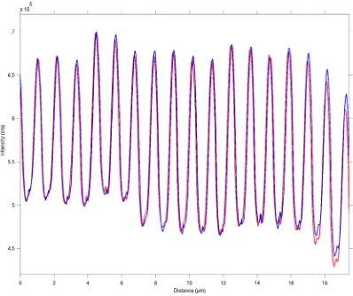
Figure 3.8: Repeat optical data acquired simultaneously to the topographical data of the phase-mask shown in Figure 3.5. The red data set relates to Figure 3.5(a) whilst the blue data set corresponds to that shown in Figure 3.5(b). The length of the scan is 19.425µm, with 1025 data points. The tip was aluminized for these measurements.
acquiring a higher count than the ‘red data’. It seems unlikely that the repeatability of this data would vary along its length, and therefore the effect is probably due to either the laser power increasing over time (each scan took about 20 minutes to complete), or increased aperture size due to loss of part of the tip’s aluminium coating.
Another example of repeated data is given in Chapter 5, Figure 5.9, where a similar length of optical data is entirely reproducible within statistical uncertainty. Interestingly, there seems to be a disturbance in the optical data of Figure 3.8 at the regions of lowest intensity. These positions correspond to the lowest part of the grating’s elevations where the associated
topographical data was also uneven. The phenomenon adds weight to the suggestion that there may be contaminants trapped within these gaps.
3.5.2 Effect Of Thermal Drift On Long-Duration, Two-dimensional Scans
A section of the optical fibre described in Table 3.1 was cleaved at both ends during an earlier stage of this project and a HeNe laser (λ=632.8) was launched into one end, via a 10x
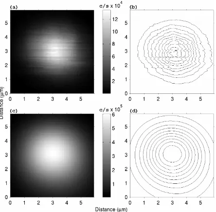
objective. Both the objective and the fibre were supported upon a Martock translation stage. The opposite end of the fibre was positioned vertically upon a metal block, directly below an aluminized SNOM tip, and held in place with a magnet. A two-dimensional image was then collected with the SNOM probe locked to the fibre’s cleaved surface, and this is shown in Figure 3.9(a). The computer data-acquisition program for this type of scan was coded in ‘C++’. The result shows substantial thermal drift, which is elucidated by its associated contour map shown in Figure 3.9(b). However, the measured profile does indicate single-mode propagation of the light, although the wavelength is slightly below the single-mode cut-off of the fibre, which is 665nm. The image was collected with less substantial SNOM polystyrene casing than that described above in Section 3.4, and without laboratory isolation. It is shown here in order to demonstrate significant improvement to the system, by its comparison to a similar image that utilizes a length of identical optical fibre, and that can be seen in Figure 3.9(c). The latter image was derived with the final polystyrene casing described above in place, and with
Figure 3.9: Two-dimensional, 1s per point, images of laser light exiting an identical optical fibre. (a) 6x6µm, 71x71 pixels, λ=632.8nm. (b) A contour map corresponding to the data
compared to the data shown in Figure 3.9(a). However, the associated contour map of the data given in Figure 3.9(d) shows a distortion of the modal shape, representing an overall shift of several hundred nanometres. This is caused again by thermal drift. The image was one of the first acquired with the final set-up of equipment described in this chapter. It was therefore recorded before any of the data presented in subsequent chapters was taken, and in fact before the data shown in Figures 3.4-3.8. Although the laboratory was isolated during the scan as in the case of most other data shown in this thesis, the image was nevertheless produced without the lab having been left for a period of time beforehand. As more measurements were made throughout this project, it was found that the laboratory sometimes required up to 24 hours of isolation in order to achieve maximum thermal stability.
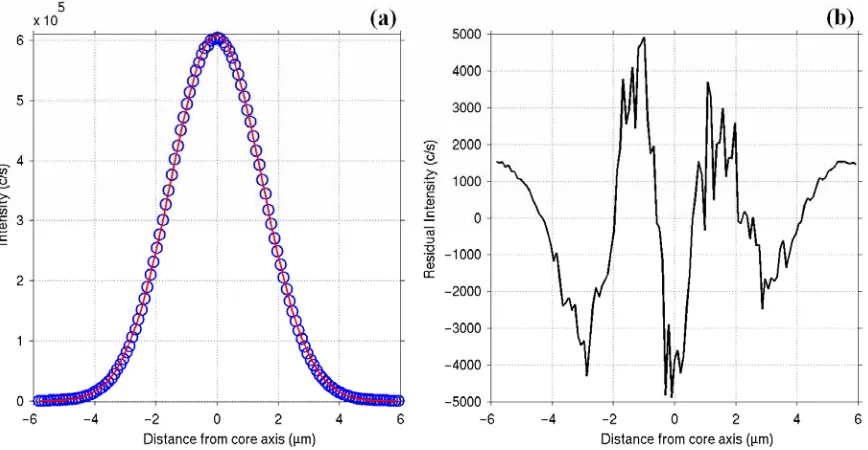
3.5.3 Mathematical Fit Of A Measured Single Mode Profile
It is unlikely that the thermal drift observed in Figure 3.9(c) had a significant affect on each individual line of data that made up the overall image. A close inspection of the figure shows the drift to be mostly in the y-direction, occurring over ~4.5 hours. The SNOM probe however, scanned in lines across the x-direction, each taking only 2 minutes to complete. A final test of the overall stability of the SNOM system and indeed the photomultiplier linearity, could therefore be performed with a mathematical fit of the single-mode profile shown in Figure 3.9(c), by using the line of data passing through the mode profile’s centre, having a total length of 11.75µm.
In the case of a true step-index optical fibre, the near-field mode profile should take the form of Bessel functions [3.15]. However, it was found that the chosen profile could be fitted more accurately to a Gaussian function. This has also been established by D.J. Butler et al during experiments under similar condit