The Use of Snyder Synthetic Hydrograph for Simulation of Overland Flow in Small Ungauged and Gauged Catchments

The Use of Snyder Synthetic Hydrograph for Simulation

of Overland Flow in Small Ungauged and Gauged Catchments

Darya FEDOROVA*, Pavel KOVÁŘ, Jan GREGAR,

Andrea JELÍNKOVÁ and Jana NOVOTNÁ

Department of Land Use and Improvement, Faculty of Environmental Sciences, Czech University of Life Sciences Prague, Prague, Czech Republic

*Corresponding author: fedorovad@fzp.czu.cz

Abstract

Fedorova D., Kovář P., Gregar J., Jelínková A., Novotná J. (2018): The use of Snyder synthetic hydrograph for simula-tion of overland flow in small ungauged and gauged catchments. Soil & Water Res., 13: 185−192.

The paper presents the results of simulated overland flow on the Třebsín experimental area, Czech Republic, using the Snyder synthetic unit hydrograph. In this research an attempt was made to discover a new approach to overland flow simulation that could give precise results like the KINFIL model for a small ungauged

catch-ment. The provided results also include a comparison with the KINFIL model for N = 10, 20, 50 and 100 year

recurrence of rainfall-runoff, with the rainfall time duration t_d = 10, 20, 30, and 60 min. Concerning a small gauged catchment, one of the most accurate and elegant methodologies, Matrix Inversion Model, can be used for the measurement of both the gross rainfall and the runoff. This method belongs to a matrix algebra concept. For the sake of completeness, we designated this model at the end of the present article to show how exact this forward march can be.

Keywords: extreme rainfall; infiltration intensity; KINFIL model; Matrix Inversion Model; Snyder unit hydrograph

One of the main problems in hydrological studies is the prediction of runoff from an ungauged basin, since the majority of small catchments are ungauged (Hrachowitz et al. 2013). The data on rainfall events are often available for such basins, however the simulation of runoff is much more complicated than for the basins with well observed data of runoff discharges. In addition, it is even more sophisticated for the small ungauged catchments (Parajka et al. 2013). There are many different approaches to the solution of such a hydrological riddle.

In 1932 the unit hydrograph method was introduced by Sherman (1932) and changed the runoff-rainfall modelling forever. It has become the most widely used method of flood analysis for gauged basins. In spite of obvious advantages, simplicity and appli-cability of this method, it has one big imperfection: it cannot be used on the basins with lack of data. For the extension of the unit hydrograph theory for

ungauged basins the synthesis from physical char-acteristics should be considered as an effective and necessary measure.

are in the used methodologies or in recognized rela-tionships (Ellouze-Gargouri & Bargaoui 2012; Singh et al. 2014; Rigon et al. 2016). Those methods for developing a synthetic hydrograph for ungauged areas have been made by Bernard (1935), Snyder (1938), McCarthy (1939) and Clark (1945).

The final step of our study was a Matrix Inversion Model calculation. The basics of this methodol-ogy were developed by Snyder (1961), through the concepts of matrices and vectors. The convolution of excess rainfall with the T-hour Unit Hydrograph (TUH) is simply the process of multiplication of a matrix by a vector.

The present study was conducted in the Třebsín experimental area. The surface runoff simulation was done using two different approaches: Snyder synthetic unit hydrograph method and kinematic wave based on the KINFIL model.

MATERIAL AND METHODS

This paper describes the continuation of research outcomes from the article published by Fedorova et al. (2017), using the HEC-HMS SCS Unit Hydrograph and KINFIL model to compute the surface runoff from extreme rainfall in the small ungauged Kninice catchment. One of the articles mentioning the unit hydrograph was published by Černohous and Kovář (2009) due to approximation of the recession limb of the hydrograph. The KINFIL model is currently used for simulating erosion processes and for predicting the vulnerability of soil to water, since the surface runoff and water erosion are closely related. In the calcula-tion, we designed rainfall events on experimental plots No. 4 and 5 in Třebsín, which are located about

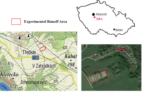
40 km from Prague in south-east direction, close to the village of Třebsín. The location of Experimental Runoff Area (ERA) is depicted in Figure 1.

In sum, there are nine experimental plots, the length of each is 36 m and the width is 7 m. The average slope of the experimental area is about 7°. The research location is operated by the Research Institute for Soil and Water Conservation in Prague-Zbraslav (RISWC Prague). The area belongs to a mildly warm region, with annual mean precipitation of 517 mm, average temperature of 6.5°C and an altitude of 340–350 m a.s.l. The natural soil composition is originally a gneiss substrate and is mostly of Haplic Cambisol type, belonging to the soil group of silty loam.

The scheme of experimental runoff plots is pre-sented in Figure 2. The studied plots are highlighted in green colour.

Rainfall data. The rainfall data from the Benešov

station was used for runoff simulation in the Třebsín catchment. This rain gauge provides daily rainfall data with a return period N = 2, 5, 10, 50 and 100 years. Due to the small catchment area, the selected pe-riods of critical rainfall time duration are t_d = 20, 30 and 60 min and the return period of N = 10, 20, 50 and 100 years. To compute the reduction in the daily rainfall depths P_t,N the DES_RAIN procedure (http://fzp.czu.cz/vyzkum) was used (Vaššová & Kovář 2011). The procedure is based on regional parameters a and c, derived by the methodology of Hrádek and Kovář (1994). The results are provided in Table 1.

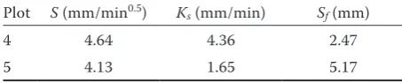
Field measurements. The average values for

satu-rated hydraulic conductivity K_s (mm/min) and for sorptivity S (mm/min0.5_{) were obtained by the}

infil-trometer method (double cylinders).

Richards’ equation (Kutílek & Nielsen 1994) combined with Philip’s solution for non-steady flow infiltration (Philip 1957) was implemented for the calculation of hydraulic soil parameters. Simplified Philip’s equation for infiltration intensity v_f calculated with saturated hydraulic conductivity K_s (m/s) and sorptivity S (m/s0.5_{) is as follows:}

(1)

Subsequently, parameters K_sand S were both com-puted, applying the non-linear regression method (Kovář et al. 2011; Štibinger 2011). Table 2 provides the measured hydraulic conductivity K_s, sorptivity S, and the storage suction factor S_f(mm):

(2)

Snyder Unit Hydrograph. The unit hydrograph

is a universal solution for any basin rainfall-runoff relationship providing the single storm hydrograph parameters given the excess rainfall data. However, a major part of watersheds has no recorded rainfall or runoff data. The answer is in the synthesis of unit

hydrographs ‒ estimating the simple rainfall-runoff relationship by application of physical parameters of drainage basin.

In 1938, a concept of the synthetic unit hydro-graph was introduced by Snyder. The methodology is based on the detailed and structured analysis of a large number of hydrographs from different catch-ments in the Appalachian region. The study led to the following formula (3) for time lag (Ponce 1989):

(3)

where:

T_lag – catchment time lag (h)

C_t – coefficient explaining the catchment gradient and related to catchment storage

L – mainstream length (km)

L_c – mainstream length from outlet to the closest point to the catchment centroid (km)

Snyder’s formula for peak discharge is as follows (Ponce 1989):

(4)

where:

Q_p – peak discharge related to 1 cm of effective rainfall (m3_/s)

A – catchment area (km2₎

C_p – empirical coefficient connected with triangular base time to time lag

KINFIL rainfall-runoff model. The KINFIL model

is used for simulation of significant rainfall-runoff events or for estimation of design discharge in catch-ments that are impacted by human activities. The kinematic wave techniques are generally considered to be sufficient for the analysis of overland and chan-nel flow. This method is a simplified version of the dynamic wave theory.

The current version of presented model consists of two parts. The first part is based on the Green-Ampt infiltration theory with ponding time accord-ing to Mein and Larson (1973) and Morel-Seytoux

Figure 2. The scheme of runoff plots

Table 1. Maximum rainfall depths P_t,N at the Benešov station (mm)

N

(years) (mm)Pt,N

t (min)

10 20 30 60

2 38.6 12.8 15.7 17.7 20.5

5 52.9 18.6 23.0 26.1 31.4

10 62.0 22.3 28.3 32.6 38.9

20 71.6 27.2 34.7 40.1 48.1

50 83.3 33.4 42.9 49.7 60.3

100 92.4 37.9 49.2 57.2 69.3

 

2

f s

v t _ S t_  _K

2

2 f

s

S S

K







lag t c

T C LL

2.78 p p

lag

C A

Q

T

 



Table 2. The soil hydraulic parameters: saturated hydrau-lic conductivity (K_s), sorptivity (S), and storage suction factor (S_f)

Plot S (mm/min0.5_{) Ks (mm/min) Sf (mm)}

4 4.64 4.36 2.47

(Morel-Seytoux & Verdin 1981; Morel-Seytoux 1982):

(5)

(6)

(7)

where:

K_s – hydraulic conductivity (m/s)

z_f – vertical extent of the saturated zone (m) θ_s – water content at natural saturation (–) θ_i – initial water content (–)

H_f – wetting front suction (m)

i – rainfall intensity (m/s)

S_f – storage suction factor (m)

t_p – ponding time (s)

t – time (s)

In small experimental catchments the hydraulic conductivity K_sand thestorage suction factor S_f can be measured directly.

The overland flow part of the model uses the kin-ematic equation and can be described by Eq. (8) (Kibler & Woolhiser 1970; Beven 2006):

(8)

where:

r_e (t) – rainfall excess intensity (m/s)

y, t, x – ordinates of the depth of water, time and posi-tion (m, s, m)

α, m – hydraulic parameters

Matrix Inversion Model. One of the most accurate

mathematical models for known rainfall and runoff parameters is the Matrix Inversion Model. The basic processes of this method have been developed in the Tennessee Valley Authority (TVA) study by Snyder (1961). The detailed view if the process involved in the convolution of discrete values of TUH with the rainfall excess to produce the direct runoff through summation is provided by Equation 9 (O’Donnell 1960):

(9)

where:

Q – runoff (m3_/s)

P – rainfall (mm/h)

U – unit hydrograph ordinates

m – number of rainfall intervals

n – number of isochrone areas (equals to the number

of TUH ordinates) ΔT – length of time period (h)

When ΔT0,then the summation can be replaced by Duhamel’s convolution integral:

(10)

where:

Q (t) – direct runoff (m3_/s)

τ – dummy time variable (−)

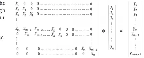
Eq. (9) shows that basically the process is the multi-plication of a matrix by a vector. However, this means to solve m+ n–1 equations of n unknown values of TUH. Consequently, it is an overdetermined system of m–1 equations and it can hardly be solved by the substitution method. This computation suits the matrix algebra very well (Figure 3):

The matrix equivalent of the equations of Figure 3 is given by Figure 4:

The matrix technique suggested in the above-mentioned TVA study (Snyder 1961) automatically provides a least-squares solution to TUH ordinates. Precipitation P should be replaced by the letter X

(only for rainfall, e.g. liquid form of precipitation);









S f f f s i f

K z H z   dz dt





f s i f

S   H

/ 1

p f

S

i

t S i

K

 

 _  _

 

 

1

α m e

y _{m y} y _{r t}

t x



 _{   } _

 

1 1

1

m n

m n m m n

Q     T



 

 





0

τ τ τ

t

Q t 

_

Figure 4. Matrix equivalent of discrete convolution equa-tions

Q by the letter Yfor discharge and the usual nota-tion, the matrix equation can be written:

|X| × |U| = |Y| (11)

To solve Eq. (11) for |'U|, one must first make the rectangular matrix |'X| a square one. This can be done by multiplying both sides of Eq. (11) by the transpose of |X|T _{left side, which is the matrix}

cre-ated by interchanging the rows and the columns of |X| in Equation 12:

|X|T _{× |X| × |U| = |Z| × |U| = |X|}T _{× |Y| (12)}

where:

|X|T _{× |X| = |Z| (13)}

|A| = |X|T _{× |Y| (14)}

|U| = |Z|–1 _{× |X|}T _{× |Y| = |Z|}–1 _{× |A| (15)}

The computed vector |U| gives the procedure find-ing the TUH ordinates directly from a gross rainfall step by step to reach a net rainfall up to a direct runoff |YC| (Y computed) using standard matrix routines:

|YC| = |X| × |U| (16)

Hidden in the manipulation of the matrix algebra on the right side of Eq. (16) is the least-squares curve fitting technique mentioned above but to repeat it to requested close coincidence with a net rainfall and T-Unit Hydrograph ordinates. The improved rainfall data is now used to find a better estimate of the TUH and the whole process is repeated.

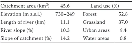
We were testing the Matrix Inversion Model on a dangerous event in the Jilovsky River catchment. The flooding occurred on 4–5 of July in 2009 (24 h) when a gross rain was falling for about 10 hours. The difference in gross and net rainfall was extremely large: 80 – 10.25 = 69.75 (mm). Table 3 provides the basic parameters of the Jilovsky catchment.

RESULTS AND DISCUSSION

The Unit Hydrograph (UH) was first proposed by Sherman (1932), originally named unit-graph.

The UH is a very simple and effective method of the rainfall-runoff simulation, however it cannot be used if there is a lack of data. In this case the synthetic unit hydrograph modifications should be used (Clark’s, Snyder’s, SCS). Since the majority of small watersheds have no recorded runoff or rainfall data, it must be a synthetic hydrograph.

Snyder (1938) presented a method of deriving synthetic unit graphs empirically. The study and analysis of rainfall-runoff characteristics were done in ungauged and gauged catchments of the Appalachian Mountains of the Eastern United States. There are two main parameters for the Snyder synthetic UH: the lag factor (C_t) and the peak flow factor (C_p). These parameters are topographically dependent and should be estimated for each particular case. In this study both those parameters were derived from measured data (Melching & Marquardt 1997; Ramírez 2000). Snyder’s method was chosen for this study also because it is a part of HEC-HMS software.

Many researches have studied the implementation of the Snyder hydrograph, since it is one of the most popular solutions for the ungauged catchments. In their research Hoffmeister andWeisman (1977) used the synthetic unit hydrograph for an ungauged basin in New Zealand. The authors simulated the run-off using three different methods: Snyder’s method, SCS dimensionless hydrograph and Commons’ di-mensionless method in six basins of two hydrological regions. The synthetic UH were compared with unit hydrographs based on observed data. The results of research show that Snyder’s method is reasonably accurate.

In Europe a good representative study of synthetic unit hydrographs was conducted in Poland, in the Grabinka catchment by Wałęga et al. (2011). The research results show that both Clark’s and Snyder’s methods are applicable, with slightly better results of Snyder’s method. The publication also contains an interesting approach to the estimation of necessary parameters for simulation.

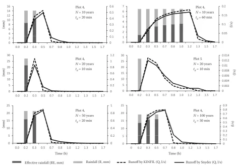
The previous study on a comparison of SCS syn-thetic unit hydrograph and KINFIL model showed that KINFIL model provided better results due to the more natural form of hydrograph. The comparison of simulated runoff by KINFIL model and Snyder’s method shows that the Snyder synthetic hydrograph improved results compared to a previous study on the SCS synthetic unit hydrograph.

Figure 5 demonstrates the results of simulation for plots 4 and 5 of the Třebsín ERA. The simulation by

Table 3. Jilovsky catchment parameters

Catchment area (km2_{) 45.6 Land use (%)}

Elevation (m a.s.l.) 730–249 Forest 52.8

Length of river (km) 11.1 Grassland 37.0

River slope (%) 10.3 Urban areas 9.4

both models was made on rainfall with recurrence interval N = 10, 20, 50, 100 years, time duration

t_d = 10, 20, 30, and 60 min.

The Matrix Inversion method was well described by Dooge and O’Kane (2003) and by Mays (2010). If the unit hydrograph is described, it can be used to

determine a direct runoff for any storm event by the Matrix Inversion method. Because of the simplicity and accuracy of this method it is quite popular in different variations and climatic conditions among hydrology engineers. The study on the Johor River in Malaysia was done by Razi et al. (2010). The

syn-Figure 5. The comparison of hydrographs simulated by KINFIL model and Snyder synthetic unit hydrograph, Třebsín Experimental Runoff Area; N − recurrence interval; t_d − time duration

Figure 6. The hydrograph computed by Matrix Inversion method 0 1 0.2 0.3 0.4 0.5 0.6 4 6 8 10 12 14 16 l/s m m Třebsín, Plot 4, N = 10 years, Td = 20 min 0 0.1 0 2

0.0 0.2 0.3 0.5 0.7 0.8 1.0 1.2 1.3 1.5 1.7 time,h Effective rainfall, RE, mm Rainfall, R, mm Q by Kinfil, l/s Q Snyder, l/s 0.05 0.1 0.15 0.2 2 3 4 5 6 7 l/s mm Třebsín, Plot 4, N = 10 years, Td = 60 min 0 0 1

0.0 0.2 0.3 0.5 0.7 0.8 1.0 1.2 1.3 1.5 1.7 time, h Effective rainfall, RE, mm Rainfall, R, mm Q by Kinfil, l/s Q Snyder, l/s 0 2 0.4 0.6 0.8 1 1.2 5 10 15 20 25 30 l/s mm Třebsín, Plot 4, N = 20 years, Td = 10 min 0 0.2 0 5

0.0 0.2 0.3 0.5 0.7 0.8 1.0 1.2 1.3 1.5 1.7

time, h Effective rainfall, RE, mm Rainfall, R, mm Q by Kinfil, l/s Q Snyder, l/s 0.004 0.006 0.008 0.01 0.012 0.014 5 10 15 20 25 30 l/s mm Třebsín, Plot 5, N = 20 years, Td = 10 min 0 0.002 0 5

0.0 0.2 0.3 0.5 0.7 0.8 1.0 1.2 1.3 1.5 1.7

time, h Effective rainfall, RE, mm Rainfall, R, mm Q by Kinfil, l/s Q Snyder, l/s 0.2 0.4 0.6 0.8 1 5 10 15 20 25 l/s m m Třebsín, Plot 4, N = 50 years, Td = 20 min 0 0.2 0 5

0.0 0.2 0.3 0.5 0.7 0.8 1.0 1.2 1.3 1.5 1.7 time, h Effective rainfall, RE, mm Rainfall, R, mm Q by Kinfil, l/s Q Snyder, l/s 0 2 0.3 0.4 0.5 0.6 0.7 0.8 0.9 5 10 15 20 25 l/s mm Třebsín, Plot 4, N = 100 years, Td = 30 min 0 0.1 0.2 0 5

0 0.2 0.3 0.5 0.7 0.8 1.0 1.2 1.3 1.5 1.7

time, h

Effective rainfall, RE, mm Rainfall, R, mm

Q by Kinfil, l/s Q Snyder, l/s

Plot 4, N = 10 years t_d = 20 min

Plot 4, N = 10 years t_d = 60 min

Plot 4, N = 20 years td = 10 min

Plot 5 N = 20 years td = 10 min

Plot 4, N = 50 years t_d = 20 min

Plot 4, N = 100 years t_d = 30 min

(mm) Time (h) (l/s) (mm) (mm) 0.2 0.4 0.6 0.8 1 5 10 15 20 25 l/s m m Třebsín, Plot 4, N = 50 years, Td = 20 min 0 0.2 0 5

0.0 0.2 0.3 0.5 0.7 0.8 1.0 1.2 1.3 1.5 1.7

time, h Effective rainfall, RE, mm Rainfall, R, mm Q by Kinfil, l/s Q Snyder, l/s 0.2 0.4 0.6 0.8 1 5 10 15 20 25 l/s m m Třebsín, Plot 4, N = 50 years, Td = 20 min 0 0.2 0 5

0.0 0.2 0.3 0.5 0.7 0.8 1.0 1.2 1.3 1.5 1.7 time, h

Effective rainfall, RE, mm Rainfall, R, mm Q by Kinfil, l/s Q Snyder, l/s

Effective rainfall (RE, mm) Rainfall (R, mm) Runoff by KINFIL (Q, l/s) Runoff by Snyder (Q, l/s)

0.2 0.4 0.6 0.8 1 5 10 15 20 25 l/s m m Třebsín, Plot 4, N = 50 years, Td = 20 min 0 0.2 0 5

0.0 0.2 0.3 0.5 0.7 0.8 1.0 1.2 1.3 1.5 1.7

time, h Effective rainfall, RE, mm Rainfall, R, mm Q by Kinfil, l/s Q Snyder, l/s 0.2 0.4 0.6 0.8 1 5 10 15 20 25 l/s m m Třebsín, Plot 4, N = 50 years, Td = 20 min 0 0.2 0 5

0.0 0.2 0.3 0.5 0.7 0.8 1.0 1.2 1.3 1.5 1.7

time, h Effective rainfall, RE, mm Rainfall, R, mm Q by Kinfil, l/s Q Snyder, l/s Time (h) (l/s) (l/s) 0 5 10 15 20 25

0 1 2 3 4 5 6 7 8 9 10 11 12 13 14 15 16 17 18 19 20 21 22 23 24 25 26 27 28 29 30 31 32 33

Time (h)

The

Matrix

Inversion

model

hydrograph

Net rainfall, mm/h Gross rainfall, mm/h Observed runoff, m3/h Computed runoff, m3/h

Net rainfall (mm/h) _{Gross rainfall (mm/h)} Observed runoff (m3_{/h) Computed runoff (m}3_/h)

thetic flood hydrographs were calculated using the SCS Unit Hydrograph method and the convolution matrix procedure.

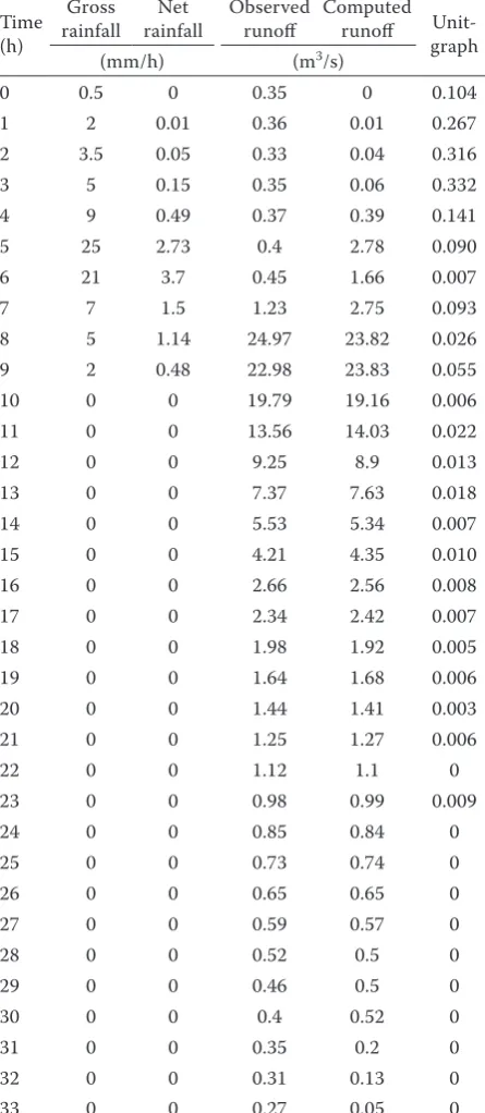
The results of the Matrix Inversion Model for the Jilovsky catchment are presented in Table 4. The calculated hydrograph is presented in Figure 6.

The successfulness of calibration and validation of models is usually described by the Nash and

Sut-cliffe Coefficient of Efficiency (CE). In the case of the maximum coincidence CE = 1.00. The equation for the Nash and Sutcliffe coefficient calculation is:

(17)

where:

Q_i – observed runoff (m3_/s)

Q_c – computed runoff (m3_/s)

Q– – mean value of observed runoff (m3_/s)

n − number of runoff ordinates

Coefficient of efficiency for the current study is CE = 0.989, which is considered to be very high. The efficiency of the Jilovsky catchment is surprisingly accurate.

CONCLUSION

Among all available models for runoff simulation in ungauged catchments different variations of the synthetic unit hydrograph take the leading place, how-ever, it was necessary to consider that there are many effective, physically based models. The previous study showed that the main disadvantage of the applied SCS synthetic unit hydrograph method was its less natural shape. Snyder’s method of the synthetic hydrograph is obviously free of this disadvantage. Nonetheless, the main difficulty is the derivation of necessary coefficients. If this problem can be solved in any manner, this method is considered to be effective for runoff simulation in ungauged catchments, yet, it needs further research on catchments under different conditions. Hydrology as a science expands quickly and a new developed technol-ogy shows the priority of physically based methods in gauged catchments. New methodology, such as various time series (Fourier series, Laguerre function, etc.) and inversion via matrices, is developed rapidly in terms of mathematical modelling.

Acknowledgements. Supported by the Czech Science Foundation as a part of Project No. IGA2017 20174257 – Modelling of the Overland Flow to Mitigate a Harmful Impact of Soil Erosion.

References

Bernard M. (1935): An approach to determinate stream flow. Transactions of the American Society of Civil Engineers, 100: 347–362.

Beven K.J. (2006): Rainfall-Runoff Modelling. The Primer. Chichester, John Wiley & Sons.

Table 4. The matrix hydrograph reconstruction

Time (h)

Gross

rainfall rainfallNet Observed runoff Computed runoff Unit-graph

(mm/h) (m3_/s)

0 0.5 0 0.35 0 0.104

1 2 0.01 0.36 0.01 0.267

2 3.5 0.05 0.33 0.04 0.316

3 5 0.15 0.35 0.06 0.332

4 9 0.49 0.37 0.39 0.141

5 25 2.73 0.4 2.78 0.090

6 21 3.7 0.45 1.66 0.007

7 7 1.5 1.23 2.75 0.093

8 5 1.14 24.97 23.82 0.026

9 2 0.48 22.98 23.83 0.055

10 0 0 19.79 19.16 0.006

11 0 0 13.56 14.03 0.022

12 0 0 9.25 8.9 0.013

13 0 0 7.37 7.63 0.018

14 0 0 5.53 5.34 0.007

15 0 0 4.21 4.35 0.010

16 0 0 2.66 2.56 0.008

17 0 0 2.34 2.42 0.007

18 0 0 1.98 1.92 0.005

19 0 0 1.64 1.68 0.006

20 0 0 1.44 1.41 0.003

21 0 0 1.25 1.27 0.006

22 0 0 1.12 1.1 0

23 0 0 0.98 0.99 0.009

24 0 0 0.85 0.84 0

25 0 0 0.73 0.74 0

26 0 0 0.65 0.65 0

27 0 0 0.59 0.57 0

28 0 0 0.52 0.5 0

29 0 0 0.46 0.5 0

30 0 0 0.4 0.52 0

31 0 0 0.35 0.2 0

32 0 0 0.31 0.13 0

33 0 0 0.27 0.05 0









2 1

2 1

1 n

i c i

n i i

Q Q CE

Q Q 



  



Černohous V., Kovář P. (2009): Forest watershed runoff changes determined using the unit hydrograph method. Journal of Forest Science, 55: 89–95.

Clark C. (1945): Storage and unit hydrograph. Transac-tions of the American Society of Civil Engineers, 110: 1419–1446.

Dooge J., O’Kane P. (2003): Deterministic Methods in Systems hydrology. IHE Delft Lecture Note Series, CRC Press. Ellouze-Gargouri E., Bargaoui Z. (2012): Runoff Estimation

for an Ungauged Catchment Using Geomorphological Instantaneous Unit Hydrograph (GIUH) and Copulas. Water Resources Management, 26: 1615–1638. Fedorova D., Bačinová H., Kovář P. (2017): Use of terraces

to reduce overland flow and soil erosion, comparison of the HEC-HMS model and the KINFIL model application. Soil and Water Research, 12: 195–201.

Hoffmeister G., Weisman R. (1977): Accuracy of synthetic hydrographs derived from representative basin. Hydro-logical Sciences, 22: 297–312.

Hrachowitz M., Savenije H., Blöschl G., McDonnell J., Siva-palan M., Pomeroy J., Arheimer B., Blume T., Clark M., Ehret U., Fenicia F., Freer J., Gelfan A., Gupta H., Hughes D., Hut R., Montanari A., Pande S., Tetzlaff D., Troch P., Uhlenbrook S., Wagener T., Winsemius H., Woods R., Zehe E., Cudennec C. (2013): A decade of predictions in ungauged basins (PUB) – a review. Hydrological Sciences Journal, 58: 1198–1255.

Hrádek F., Kovář P. (1994): Computation of design rainfalls. Vodní hospodářství, 11: 49–53. (in Czech)

Kibler D.F., Woolhiser D.A. (1970): The Kinematic Cascade as a Hydrologic Model. Hydrology Paper No. 39, Fort Collins, Colorado State University.

Kovář P., Vaššová D., Hrabalíková M. (2011): Mitigation of surface runoff and erosion impacts on catchment by stone hedgerows. Soil and Water Research, 6: 153–164. Kutílek M., Nielsen D. (1994): Soil Hydrology.

Cremlingen-Destedt, Catena Verlag: 98–102.

Mays L. (2010): Water Resources Engineering. 2nd _{Ed. New} York, John Wiley and Sons, Inc.

McCarthy G. (1939): The Unit Hydrograph and Flood Rout-ing. Providence, US Corps of Engineers Office. Mein R.G., Larson C.L. (1973): Modelling infiltration

dur-ing a steady rain. Water Resources Research, 9: 384–394. Melching C., Marquardt J. (1997): Equations for Estimating Synthetic Unit-Hydrograph Parameter Values for Small Watersheds in Lake County, Illinois. Urbana, Open-File Report, US Geological Survey.

Morel-Seytoux H.J. (1982): Analytical results for prediction of variable rainfall infiltration. Journal of Hydrology, 59: 209–230.

Morel-Seytoux H.J., Verdin J.P. (1981): Extension of the SCS Rainfall Runoff Methodology for Ungaged Watersheds.

[Report FHWA/RD-81/060.] Springfield, US National Technical Information Service.

O’Donnell T. (1960): Instantaneous Unit Hydrograph Deri-vation by Harmonic Analysis. IASH Publication No. 51, Commission of Surface Waters: 546 – 557.

Parajka J., Viglione A., Rogger M., Salinas J.L., Sivapalan M., Blöschl G. (2013): Comparative assessment of predictions in ungauged basins – Part 1: Runoff-hydrograph studies. Hydrology and Earth System Sciences, 17: 1783–1795. Philip J.R. (1957): The theory of infiltration. The

infiltra-tion equainfiltra-tion and its soluinfiltra-tion. Soil Science, 83: 345–357. Ponce V.M. (1989): Engineering Hydrology: Principles and Practices. Englewood Cliffs, Prentice Hall Upper Saddle River.

Ramírez J.A. (2000): Prediction and Modelling of Flood Hydrology and Hydraulics. Chapter 11. In: Wohl E. (ed.): Inland Flood Hazards: Human, Riparian and Aquatic Communities. New York, Cambridge University Press: 293–329.

Razi M.A., Ariffin J., Tahir W., Arish N.A. (2010): Flood Estimation Studies using Hydrologic Modelling System (HEC-HMS) for Johor River, Malaysia. Journal of Applied Sciences, 10: 930–939.

Rigon R., Bancheri M., Formetta G., de Lavenne A. (2016): The geomorphological unit hydrograph from a historical-critical perspective. Earth Surface Processes and Land-forms, 41: 27–37.

Sherman L.K. (1932): Stream flow from rainfall by the unit hy-drograph method. Engineering News Record, 108: 501–505. Singh P.K., Mishra S.K., Jain M.K. (2014): A review of the

synthetic unit hydrograph: from the empirical UH to advanced geomorphological methods. Hydrological Sci-ences Journal, 59: 239–261.

Snyder F. (1938): Synthetic unit-graphs. Eos, Transactions, American Geophysical Union, 19: 447–454.

Snyder F. (1961): Study of the Tennessee Valley Author-ity. Matrix Operation in Hydrograph Computations. Research Paper 1, Knoxville, Office of Tributary Area Development.

Štibinger J. (2011): Infiltration capacities. Stavební obzor, 2/2011: 78–83. (in Czech)

Vaššová D., Kovář P. (2011): DES_RAIN, Computational Program. Prague, FZP CZU.

Wałęga A., Grzebinoga M., Paluszkiewicz B. (2011): On us-ing the Snyder and Clark unit hydrograph for calculations of flood waves in a highland catchment (the Grabinka river example). Acta Scientiarum Polonorum, Formatio Circumiectus, 10: 47–56.