Fast numerical simulation of vortex shedding in tube arrays using a discrete vortex method

Fast numerical simulation of vortex shedding in tube arrays using a discrete vortex method

C. Sweeney and C. Meskell

Department of Mechanical Engineering, Trinity College, Dublin, Ireland.

Published in Journal of Fluids and Structures, 18 (2003) 501-512, doi:10.1016/j.jfluidstructs.2003.08.009

Abstract

1 Introduction

Weaver (1987) notes that if periodicity exists in the flow in the absence of structural motion then “self-controlled vibrations” may occur. Thisflow periodicity may be generated by acoustic resonance or by an-other mechanism referred to as Strouhal periodicity. Both mechanisms will produce similar tube responses, a fact that led Weaver & Fitzpatrick (1988) to dismiss as unreliable much earlier (pre1980) Strouhal data for tube arrays, since it was obtained from heat exchangers prone to acoustic resonance.

Prior to the 1960s, vortex shedding within heat exchangers (which was thought to be identical to that from a single cylinder) was accepted as the major cause of FIV in tube bundles. But Owen (1965) disputed the possiblity that discrete vortex shedding could occur in closely packed tube arrays. He attributed the widely observed resonant phenomenon to a peak in the turbulence spectrum, the frequency of which was dependent on flow velocity and array geometry. He derived a semi-empirical formula to predict the frequency of this peak. Paidoussis (1981) pointed out that other predictive formulae, which were based on the vortex shedding concept, agreed well with Owen’s model. He argued that, since the various semi-empirical formulae were based on the same experimental data, it was hardly surprising that the predictions were comparable.

However, Owen’s ideas highlight the fact that even at the time of Paidoussis’ review (1981), there was no definitive proof of the exact nature of Strouhal periodicity, as the phenomenon had come to be known. For example, Grover & Weaver (1978), despite setting out to clarify the issue, succeeded only in observing a strong resonant peak in tube response, the existance of which was not in doubt. It was not until 1985, that Weaver & Abd-Rabbo (1985) published a flow visualization study of water flow in a fullyflexible, normal square (inline) array (P

d = 1.5), which shows periodic vortex shedding, although not very clearly. Several other visualization studies followed for various array geometries. Price et al. (1992) show pictures of vortex shedding in a parallel triangular array (P

d = 1.375); Weaver et al. (1992) present photographs of vortex shedding in rotated square arrays (P

d = 1.21to1.83) with air as the workingfluid. Perhaps the clearest images of vortex shedding have been produced by Oengeron & Ziada (1998) who investigated both inline and staggered array configurations subject to water crossflow including several normal triangular arrays.

Before the acceptance of vortex shedding as the mechanism of Strouhal periodicity, much was known about the phenomenon. Weaver & Yeung (1984) having studied all four array geometries, produced a general expression which relates the RMS tube response, normalized against tube diameter, to the mass damping parameter (including “fluid added mass”). The authors suggest that vortex shedding will not produce significant tube response for mass damping parameters greater than about unity, although they caution that the experimental data is quite sparse.

Savkar (1984) reported that upstream turbulence generators (grids) in air flow eliminated the problem of Strouhal periodicity altogether. This result suggests that, since turbulence levels by thefifth row are very high (Weaver & El-Kashlan, 1981), the problem of Strouhal periodicity is only a problem in thefirst few rows. However, Fitzpatrick et al. (1986) report a substantial peak in the turbulence spectra as deep as the fifteenth row of inline arrays. They also reported multiple Strouhal numbers. This result has been found by other researchers. Paidoussis et al. (1988) found two Strouhal numbers for a rotated square array, P

Price et al. (1987) report three Strouhal numbers, but note that only one Strouhal number persists beyond the fourth row.

Previously, Zukauskas & Katinas (1980) attempted to collapse all the Strouhal data on to a single curve,

however, the presence of multiple vortex shedding frequencies renders their curve obsolete. Polak & Weaver (1995) argue that for normal triangular arrays with a pitch ratio of less than 2, only a single shedding frequency

can be observed. However, Oengoren & Ziada (1998) collated all the available data, including new data from their own study, to provide two empirical curves which predict the Strouhal number as a function of pitch ratio. Furthermore, they go on to show experimentally that the higher value is dominant at small pitch ratios (P

d < 1.6), while the lower Strouhal number dominates in arrays with large pitch ratios (Pd >3.4). At intermediate spacing, both Strouhal numbers are apparent, but which is strongest depends on which row is being examined, and in some cases, how many tubes are in a row. The presence of a third shedding frequency can be attributed to a non-linear interaction between the other two frequencies. This explains the behaviour reported by Price et al. (1987).

As can be seen from the discussion above, vortex shedding in tube arrays is now reasonably well under-stood. However, it is also clear that this knowledge base has been achieved primarily through experimental investigation.

The steady state mass and heat transfer in heat exchanger tube bundles have been successfully modelled numerically by making use of the periodic nature of the geometry (e.g. Johnson et al., 1993; Beale & Spalding, 1998). Beale & Spalding (1999) have also employed periodic boundaries with a finite volume discretisation of the laminar Navier-Stokes equations cast in primitive variables to simulate the unsteady flow in rigid tube arrays and so obtain Strouhal numbers. They state that “ideally,flow-field calculations would be performed over the entire bank of tubes”, but note that computational restrictions on the mesh size and density make this impractical for this method of flow simulation. There have also been studies which have applied large eddy simulation (LES) to a full tube array (e.g. Barsamian & Hassan, 1997). However, LES is still very costly computationally, and so is not useful as a potential design tool nor as a tool for parametric studies.

2 Governing equations

The governing equations which are needed to describe two dimensional, incompressiblefluidflow may be expressed as the vorticity transport equation, Eq. (1), and the stream function-vorticity equation, Eq. (2).

∂ω ∂t =

−∂ψ

∂y ∂ω ∂x +

∂ψ ∂x

∂ω ∂y

C

+

ν

∂2ω ∂x2 +

∂2ω ∂y2

D

(1)

∇2_{ψ =−ω (2)}

whereψis the stream function,ωis the vorticity andνis the dynamic viscosity.

Vortex methods use a Lagrangian approach toflow simulation by concentrating on the vorticityfield in the flow. If thefield is represented by point vortices, then the governing equations of theflow may be solved by considering the creation, interaction and motion of these point vortices.

Chorin (1973) proposed an operator-splitting scheme whereby the processes of convection and viscous diffusion, denoted by the suffices C and D respectively, are solved separately. Convection is solved by

moving the point vortices in the velocityfield. Viscous diffusion is solved by walking the point vortices through a distance chosen at random from a Gaussian distribution with standard deviation √2νΔt. The

final position of each point vortex at the end of a time step is given by the combination of the diffusion and convection processes. The simulation then advances onto the next time step, and the new velocityfield is calculated and the boundary conditions applied. This time-stepping procedure by which the governing equations are solved is called the random vortex method.

The velocityfield must be calculated by solving the stream function-vorticity Poisson equation at each time step of the simulation so that the point vortices may be convected. To solve this using a direct Biot-Savart summation for the interaction ofN point vortices would take an operation count ofO(N2).

Christiansen (1973) introduced the cloud-in-cell (CIC) method to allow a more efficient calculation of the velocityfield. In this method, a mesh is placed over theflowfield and the vorticity of the point vortices is attributed to the nodes of the cell in which it is contained. Once all of the point vortices have been spread in this way onto the nodes of the mesh, the governing stream function - vorticity equation can be solved on the mesh using standard Eulerian mesh techniques, such asfinite-difference. The velocity of each point vortex in thisflowfield can be now obtained from the stream functions at the mesh points by interpolation, and the simulation advanced.

This reduces the cost of theflowfield calculation forN point vortices fromO(N2)(calculating the effect

of every point vortex on every other point vortex) to a number of computations that is roughly linear in the number of vortices and mesh points,O(N +M)(Milinazzo & Saffman 1977). Although this method

The objective of the cloud-in-element method is to allow the efficiencies offered by CIC to be applied for use on an unstructured mesh. This would allow an efficient calculation of the velocityfield on a single mesh due to a set of point vortices in a domain which may contain multiple bodies and complex geometries.

3 Cloud-in-element

If the velocityfield is to be solved on an unstructured mesh, the circulation of the point vortices must be spread onto the nodes of the mesh. Once this has been done, the stream function at the mesh nodes may be calculated by use of thefinite element method. There are two stages involved in preparing the mesh to calculate the velocityfield. First, each point vortex needs to be located in the mesh. This involvesfinding which triangularfinite element of the mesh contains each point vortex. Once the point vortices have been located in theirhomeelements, the strength of the point vortices must be assigned to the mesh nodes, so

that the velocityfield can be calculated.

3.1 Graphical look-up matrix

Locating a point in a regular polar or Cartesian mesh is a simple procedure, as the coordinates of the point may be used as a pointer to the mesh cell in which it belongs. It is not so easy to locate points in an unstructured mesh, however, as the elements are not necessarily regular in size, orientation, or numbered in a regular manner. It would be convenient to be able to use the coordinates of the point vortex as a pointer to its home element. This can be achieved by building a matrix which reports the likely home element for the coordinates of a given point vortex, called agraphical look-upmatrix.

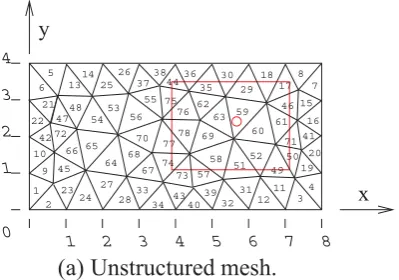
To see how a graphical look-up matrix may be used to locate a point in an unstructured mesh, consider Figure 1(a), which shows a point vortex located in element number 59 in an unstructured mesh. The graphical look-up matrix has been generated for this mesh by stepping through the unstructured mesh by a fixed amount, and at each step entering the number of that location’s home element as an index into a matrix. As the mesh does not change during the course of the simulation, neither does the graphical look-up matrix, and it can be assembled at the pre-processing stage and stored for use during the simulation. With the graphical look-up matrix, the index states the element number which contains the point at that location. This allows the coordinates of the point vortex, once suitably truncated, to be used as pointers to the row and column indices of the graphical look-up matrix, hence returning the number of the most likely home element of the point vortex, Figure 1(b).

The graphical look-up matrix offers an efficient way of getting the home element of a point in an un-structured mesh. However, if the point lies near the boundary separating two or more elements, the home element returned from the look-up matrix may be incorrect. To find out if the element number given is indeed the home element of that point, a rigorous mathematical test for determining whether a point lies inside a given triangle is required. The vector product can be used as such a test.

x y

1 2 3 4 5 6 7 8

0 1 2 3 4 5 13 14 25 26 37 6 38 4436 35 30 16 20 32 31 39 40 43 34 33 23 2 1 9 66 10 42 22 21 47 72 65 54 48 53 56 55 75 76 78 77 68 70 69 63 62 52 49 50 71 46 60 61 59 29 18 17 8 7 15 41 19 4 3 11 12 51 58 57 73 74 67 64 27 28 24 45

(a) Unstructured mesh.

44 44 36 35 35 35 35 30 29 29 29 29 18 18 17 17 75 76 76 62 62 62 62 59 59 59 29 29 29 17 46 46 76 76 76 62 62 63 63 63 59 59 59 60 60 61 61 61 78 78 78 78 63 63 63 63 59 59 59 60 60 61 61 61 78 78 78 69 69 69 63 63 59 59 60 60 60 60 81 81 77 78 78 69 69 69 69 69 59 60 60 60 60 60 61 71 77 78 78 69 69 69 58 58 51 52 52 52 52 52 71 71 77 77 69 69 58 58 58 58 51 51 52 52 52 52 49 50 74 74 57 58 58 58 58 58 51 51 52 52 52 49 49 50 74 73 73 57 58 58 58 51 51 51 51 52 52 49 49 49 73 73 73 57 57 57 58 51 51 51 51 51 49 49 49 49 75 75 62 35 35 35 35 30 29 29 29 29 18 18 17 17 76 76 76 62 62 62 63 63 59 59 59 59 60 61 46 46

(b) Graphical look-up matrix.

Fig. 1. Point location.

the element, which results in the element being positioned with the vortex at the origin. The vertices of the triangle can now be considered as vectors (a,b, c)from the point vortex to the vertices. If the vortex

is inside the triangle, thena×b,b ×candc×a will all have the same sign, as the angles between the

vectors are all less thanπ. If the vortex is outside the triangle, on the other hand, one of the cross products

will have the opposite sign to the others, as one of the angles will be greater thanπ.

This test is mathematically sufficient to verify that a point lies within a triangular element. If it is found that the point vortex doesnotlie within the element given by the graphical look-up matrix, theneighbours

matrix is used tofind the correct home element.

3.2 Neighbours matrix

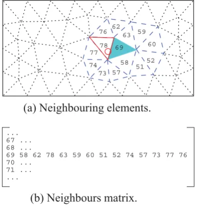
Figure 2 shows a point vortex near the edge of an element. The graphical look-up matrix returns the home element of this point as being the adjacent shaded element (#69), instead of the true home element (#78).

76 78 77 69 63 62 52 60 59 51 58 57 73 74

(a) Neighbouring elements.

... 67 ... 68 ...

69 58 62 78 63 59 60 51 52 74 57 73 77 76 70 ...

71 ... ...

(b) Neighbours matrix.

Fig. 2. Finding the correct home element.

the elements listed in row 69 of the neighbours matrix, element number 78 will be found as the true home element.

3.3 Spreading the circulation

At this stage of the process every point vortex has had its home element verified. In order to solve for the velocityfield caused by these point vortices, their circulation needs to be spread from the point vortices onto the nodes of their home elements. Then the Poisson equation can be solved on the unstructured mesh using thefinite element method to obtain the stream function and hence the velocityfield.

Area-weighting is efficient to implement with a regular Cartesian or polar coordinate system as the ratio of the areas involved can be directly related to the coordinate system being used. When spreading onto the nodes of a triangular element in an unstructured mesh, these regular coordinate systems do not directly give information about the areas needed for area-weighting. A coordinate system based on the triangle itself is desirable, and can be achieved by using area coordinates.

⎛ ⎜ ⎜ ⎜ ⎜ ⎜ ⎝ L1 L2 L3 ⎞ ⎟ ⎟ ⎟ ⎟ ⎟ ⎠= 1 2A123

⎡ ⎢ ⎢ ⎢ ⎢ ⎢ ⎣

a1 b1 c1

a2 b2 c2

a3 b3 c3

1 1

2 2 3 3

A

A

1

3

A2

1 (x ,y )

2 (x ,y ) 3 (x ,y )

P (x,y)

Fig. 3. Area-weighting in a triangle.

a1=x2y3−x3y2

b1=y2−y3 (4)

c1=x3 −x2

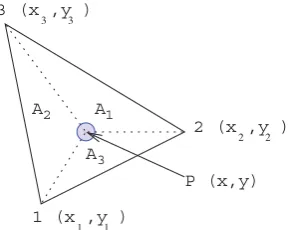
with cyclic rotation of indices1,2,3. If the circulation of the vortex atP in Figure 3 isΓ, then the

circula-tion spread onto node1will equalΓA1

A, that spread onto node2will equalΓAA2, and for node 3 will equal

ΓA3

A, whereAis the area of the triangle. Area coordinates directly give the area ratios required for area-weighting, and so the circulation spread onto node1is given byL1Γ, the circulation on node2isL2Γ, and

for node 3isL3Γ. Once the circulation has been assigned onto the nodes of the unstructured mesh in this

manner for all the point vortices, thefinite element method is used to solve the stream function-vorticity equation, and the velocityfield is obtained.

3.4 Boundary considerations

Any solid surfaces in a viscousflow require two boundary conditions to be enforced. The zero-permeability boundary condition ensures that thefluidflowsaroundand notthroughthe solid. If there is only a single

body in theflow, a Dirichlet condition may be applied by setting the value of the stream function at the solid surface to a constant. If there is more than one body in theflow, the stream function values for the different bodies will not be known in advance. In this case a source panel method can be used to enforce a Neumann condition of zero normal flux at the surface. In the source panel method the strengths of a collection of source panels is calculated from the onset velocity and the geometries of the solid surfaces so as to ensure that theflow does not cross the boundary (Kellogg, 1929).

Another boundary condition which must be applied is the no-slip condition. The velocity of the fluid at the surface is zero, as viscosity causes thefluid to stick to the solid surface. In the simulation, the no-slip condition is enforced at the surface at each time step by creating a vortex sheet. The strength of the vortex sheet is calculated so that it will induce a velocity equal and opposite to the tangential velocity of thefluid at the surface. The overall velocity at the surface once the vortex sheet has been created, therefore, will be zero and the no-slip condition satisfied. This vortex sheet is then discretised into point vortices which diffuse into theflow.

time step, or diffusion by random walk. These internal point vortices may be absorbed following the method of Smith & Stansby (1989). Any internal point vortices are deleted, but their circulation is noted. The circulation of all internal point vortices is then assigned to the surface, and thus included in the next velocity field calculation. The no-slip condition is enforced by the creation of a vortex sheet, and new point vortices are created with circulation strengths defined by the circulation absorbed by deleted point vortices, and the circulation due to the vortex sheet enforcing no-slip.

4 Validation for one cylinder

In order to validate the cloud-in-element method, simulations were run for the standard case offlow over a single circular cylinder for a range of Reynolds numbers from 40 to 9,500. Plots of the computed Strouhal number and mean drag variation with Reynolds number are compared with experimental results obtained from the review onflow around circular cylinders by Zdravkovich (1997) and Norberg (2001).

Figure 4 shows a good agreement between the Strouhal (St) number calculated in the present work and

experimental results. The Strouhal number increases from a low value for low Reynolds numbers, to reach a reasonably level value fromRe= 550−9500.

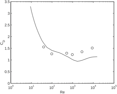
Figure 5 shows a comparison between computed and experimental results (Zdravkovich 1997) for the total mean drag (CD). The simulations show a good initial trend, the mean drag decreasing with increasing Reynolds number, and predicting values close to those found experimentally, although the agreement deteriorates somewhat at higher Reynolds numbers.

5 Application to tube array

The validated technique has been applied to a four row normal triangular array with a pitch ratio of 1.6. A schematic of the geometry can be found infigure 6. The array is similar to that investigated experimentally by Polak & Weaver (1995), the difference being that the simulation is executed using non-dimensional units with a tube radius is 1 and a flow velocity of 1. The simulation time is also non-dimensional. The Reynolds number is set by the value of the viscosity. The results can be easily scaled to represent data from a particular physical array, as long as the Reynolds numbers agree.

The computational domain, and hence the unstructured mesh, is extended slight above and below the array so as to ensure that vortices which are convected or diffused across the solid boundary can be dealt with and returned to the flow. Similarly, the mesh extends through the tubes to allow a whole field velocity calculation as required by the source panel method. This also facilitates the absorption and reintroduction of point vortices which have crossed cylinder surface. This highlights the fact that the unstructured mesh on which thefinite element solution of the velocityfield is obtained is not coincident with thefluid domain.

101 102 103 104 0.1

0.12 0.14 0.16 0.18 0.2 0.22 0.24 0.26

Re

St

Fig. 4. Mean Strouhal:◦, present work; —, experiment, Norberg (2001).

100 101 102 103 104 105

0 0.5 1 1.5 2 2.5 3 3.5

Re CD

Fig. 5. Mean drag coefficient:◦, present work; —, experiment, Zdravkovich (1997).

which corresponds to that used by Polak & Weaver in their flow visualisation, thus allowing direct com-parison with that experimental study. The simulation was initiated with a potentialflow solution in thefirst time step and was allowed to run for 2000 time steps. The non-dimensional time step was set at 0.01 giving afinal non-dimensional time (T∗ =Ut/r) of 20. As will be seen below, this corresponds to approximately

12 vortex shedding periods.

5.1 Results

The instantaneousfluid velocity was examined at the location in the second row indicated infigure 6. This is close to one of the locations of the hotwire measurements in Polak & Weaver’s study thus allowing direct comparison with experimental data. The time history of the streamwise velocity component at the location can be seen in figure 7. Since the simulation represents impulsively startedflow through a tube array, the velocityfield initially exhibits a transient build-up of vorticity (T∗ < 2), after which the trace

U

∞ _P

d

Measurement point

Fig. 6. Schematic of tube array geometry.

0 5 10 15 20

2 3 4 5 6

Non−dimensional time t*

Streamwise velocity, u

Fig. 7. Time record of streamwise velocity component in second row.

0 5 10 15 20

−2

−1.5

−1

−0.5 0 0.5

Non−dimensional time t*

Crossflow velocity, v

Fig. 8. Time record of crossflow velocity component in second row.

0 2 4 6 8 10

0 20 40 60 80

Strouhal number (St=fd/U

∞)

Power spectrum (arbitrary scale

)

St=1.27

(a) Non-dimensional time,T∗ = 6.0 (b) Non-dimensional time,T∗ = 6.2

(c) Non-dimensional time,T∗ = 6.4 (d) Non-dimensional time,T∗ = 6.6

(e) Non-dimensional time,T∗ = 6.8 (f) Non-dimensional time,T∗= 7.0

Fig. 11. Mean vorticity downstream offirst row.

Fig. 12. Variation of runtime per iteration with number of vortices.

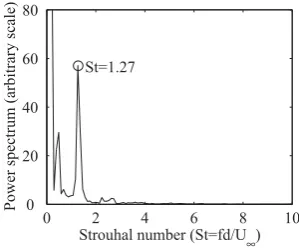
The periodic nature of the flowfield can more easily be seen in the power spectrum of the streamwise velocity shown infigure 9. The frequency has been converted to Strouhal number(St=f d/U∞). Note that the Strouhal number used here is based on the freestream velocity, as was the case in Polak and Weaver’s study, rather than on the gap velocity as was done by Oengeron & Ziada (1998). The vertical axis is an arbitray linear scale of Power Spectral Density. A strong peak is apparent in the PSD at a Strouhal number of 1.27. For a Reynolds number of 2200, Polak & Weaver reported a value for the Strouhal number based on hotwire measurements of1.2±0.15, which means that the numerical simulation has overestimated the

shedding frequency by about 6%. Although Polak and Weaver only reported a single shedding frequency for this array geometry, Oengeron and Ziada reported two discrete frequencies. The second, should be located at a Strouhal number of approximately 1.8. There is no evidence in this data for a second frequency, however, there is insufficient data in the time record to generate an averaged spectrum and obtain improved frequency resolution.

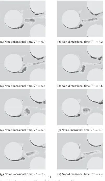
The periodic vortex shedding in the tube array predicted by the simualtion can be seen qualitatively by examining the development of the vorticityfield. Figure 10 shows the evolution of the vorticityfield behind thefirst row of the array fromT∗ = 6.0toT∗ = 7.4which corresponds to just over one vortex shedding

The sequence begins infigure 10(a) with a concentration of vorticity just detached from the leading tube. A new vortex has already started to form on the lower suface of the tube. The detached vortex is elongated as the flow is accelerated through the gap between the cylinders of the second row as can be seen in figure 10(b-d). While this detached vortex is stretched and convected downstream, the vortex which is still attached to the cylinder in thefirst row continues to grow. This vortex remains in the vicinity of thefirst row (figure 10(e,f) ) until it isfinally shed (figure 10(g) ) and begins to become elongated (figure 10(h) ). Comparison of the sequence withfigure 4 of Polak & Weaver’s study suggests that the unsteadyflowfield obtained from the simulation agrees qualitatively with experimentalflow visualization.

Figure 11 shows the absolute mean value of the vorticityfield, averaged fromT∗ = 2→20in the region

of thefirst row. As would be expected the meanflow is strongly symmetric. Thefigure shows clearly the primary recirculating regions in the wake of the first row cylinder. Interestingly, secondary recirculating regions can also be seen between the primary vortices and the tube surface.

5.2 Computational cost.

The simulation described above was executed on a desktop PC with a single Pentium 4 processor and 256 Mb of memory. The total runtime was approximately 70 minutes. New vortices are created at every time step, however, as these move downstream they are combined or deleted and so the total number of vortices being tracked in the simulation reaches a plateau which depends primarily of the size of problem considered. For this simulation a maximum of105_{vortices was used.}

Figure 12 shows the variation of the runtime for a single iteration of the algorithm with the number of vortices. As can be clearly seen, this variation is linear; i.e. the scheme is O(N), where N is the

num-ber of vortices. The velocity calculation is a constant computational overhead for a given mesh, which explains why the curve does not pass through the origin (i.e. for zero vortices the run time will not be zero). This implies that the algorithm can be applied directly to larger problems (i.e. bigger arrays) with a computational cost which is directly proportional to the size of the problem.

6 Conclusions

A variant of the Cloud-in-Cell discrete vortex method has been described which can easily accommodate the complex geometry of a tube array. This is achieved using a finite element, rather than a finite dif-ference, scheme on an unstructured mesh in order to solve for the flowfield induced by the translating point vortices. The computational problem of spreading the circulationfield represented by the cloud of vortices onto the unstructured mesh is accelerated using a look-up table. The resulting method referred to as the “Cloud-in-Element” method is computationally inexpensive for solving unsteady flow around complex bluff body geometries at moderate Reynolds number. The technique is shown to be accurate for the standard case offlow around a single circular cylinder.

Reynolds number of 2200. This case was chosen for direct comparison with experimental data available in the literature. The simulation successfully predicted the Strouhal number to within 6% of the experimental value and vortex shedding similar to that seen in experimentalflow visualization has been observed.

As the simulation was initiated effectively from quiescentfluid (i.e. startingflow) it is desirable to extend the computation in order to verify that a dynamically stable vortex shedding cycle has in fact been estab-lished and that the velocity data at any given point becomes periodic about a mean value. Furthermore, given the quantity of data available in the literature for vortex shedding in tube arrays, a detailed compari-son of dependence of the predicted Strouhal number on Reynolds number, pitch ratio and array pattern is necessary to further validate the approach.

Nonetheless, the technique provides a computationally inexpensive way to solve for the unsteady flow within an entire tube array and it offers the opportunity to explore the effects of novel array geometries without the expense and complexity of experimentation.

Furthermore, given that the approach used is basically a Lagrangian technique and that solid bodies are represented using a surface integral technique, it is in principle straight forward to extend the method to include moving boundaries.

References

Barsamian, H. & Hassan, Y. (1997). Large eddy simulation of turbulent crossflow in tube bundles.

Nuclear Engineering and Design 172, 103–122.

Beale, S. & Spalding, D. (1998). Numerical study of fluid flow and heat transfer in tube banks with stream-wise periodic boundary conditions.Transactions of CSME 22(4A), 397–416.

Beale, S. & Spalding, D. (1999). A numerical study of unsteadyfluidflow in in-line and staggered tube banks.Journal of Fluids and Structures 13, 723–754.

Chorin, A. J. (1973). Numerical study of slightly viscousflow.Journal of Fluid Mechanics 57(4), 785–

796.

Christiansen, J. P. (1973). Numerical simulation of hydromechanics by the method of point vortices.

Journal of Computational Physics 13, 363–379.

Cottet, G. & Koumoutsakos, P. (2000). Vortex methods - theory and practice. Cambridge University

Press.

Fitzpatrick, J., Donaldson, I., & McKnight, W. (1986). The structure of the turbulence spectrum of flows in deep tube array models. In C. et al. (Ed.),Flow-induced vibration, Volume PVP Vol 104,

pp. 21–30.

Grover, L. & Weaver, D. (1978). Cross-flow induced vibrations in a tube bank - vortex shedding. Jour-nal of Sound and Vibration 59(2), 263–276.

Johnson, A., Tezduyar, T., & Liou, J. (1993). Numerical simulation of flows past periodic arrays of cylinders.Computational mechanics 11, 371–383.

Kellogg, O. D. (1929).Foundations of potential theory. New York: Ungar.

Milinazzo, F. & Saffman, P. G. (1977). The calculation of large reynolds number two-dimensionalflow using discrete vortices with random walk.Journal of Computational Physics 23, 380–392.

Structures 15, 459–469.

Oengoren, A. & Ziada, S. (1998). An in-depth study of vortex shedding, acoustic resonance and turbu-lent forces in normal triangle tube arrays.Journal of Fluids and Structures 12(6), 717–758.

Owen, P. (1965). Buffeting excitation of boiler tube vibration. Journal of Mechanical Engineering Science 7, 431–439.

Paidoussis, M. (1981). Fluidelastic vibration of cylinder arrays in axial and crossflow: state of the art.

Journal of Sound and Vibration 76(3), 329–360.

Paidoussis, M., Price, S., Nakamura, T., Mark, B., & Njuki, W. (1988). Flow induced vibrations and instabilities in a rotated square cylinder array in crossflow. In Vol 2, Flow induced vibration and noise in cylinder arrays, pp. 111–138. ASME symposium offlow induced vibration.

Polak, D. R. & Weaver, D. (1995). Vortex shedding in normal triangular tube arrays.Journal of Fluids and Structures 9, 1–18.

Price, S., Paidoussis, M., MacDonald, R., & Mark, B. (1987). The flow-induced vibration of a single flexible cylinder in a rotated square array of rigid cylinders with pitch-to-diameter ratio of 2.12.

Journal of Fluids and Structures 1, 359–378.

Price, S., Paidoussis, M., & Mark, B. (1992). Flow visualization in a 1.375 pitch-to-diameter parallel triangular array subject to crossflow. InVol. 1, FSI/FIV in cylinder arrays in cross-flow, pp. 29–38.

ASME international symposium onflow induced vibrations.

Savkar, S. (1984). Buffeting of cylindrical arrays in crossflow. InVol. 2, Vibration of arrays of cylinders in crossflow., pp. 195–210. ASME symposium onflow induced vibrations.

Smith, P. A. & Stansby, P. K. (1989). An efficient surface algorithm for random-particle simulation of vorticity and heat transport.Journal of Computational Physics 81, 349–371.

Weaver, D. (1987).An introduction to Flow-induced vibrations. Course notes. BHRA.

Weaver, D. & Abd-Rabbo, A. (1985). A flow visualization study of a square array of tubes in water crossflow.Journal of Fluids Engineering 107, 354–363.

Weaver, D. & El-Kashlan, M. (1981). On the number of tube rows required to study cross-flow induced vibrations in tube banks.Journal of Sound and Vibration 75(2), 265–273.

Weaver, D. & Fitzpatrick, J. (1988). A review of cross-flow induced vibrations in heat exchanger tube arrays.Journal of Fluids and Structures 2, 73–93.

Weaver, D., Lian, H., & Huang, X. (1992). Vortex shedding in rotated square arrays. InVol. 1, FSI/FIV in cylinder arrays in cross-flow, pp. 39–54. ASME international symposium onflow induced

vibra-tions.

Weaver, D. & Yeung, H. (1984). The effect of tube mass on theflow induced response of various tube arrays in water.Journal of Sound and Vibration 93(3), 409–425.

Zdravkovich, M. M. (1997).Flow around circular cylinders, Volume 1. Oxford University Press.