Abstract—The modeling of magnetic components for use
in electrical circuit simulation requires that the core material be accurately characterized. This paper investigates a method of extracting parameters to model the hysteresis behavior of magnetic core materials and optimizing them to achieve accurate results during circuit simulation. Metrics are defined to measure specific features of the behavior of both the core magnetic material and the magnetic component, such as a transformer. This paper presents a method of applying these metrics for the purposes of comparison and optimization and demonstrates the method using measured results and corresponding simulations. It compares the effectiveness of a weighted metrics function with that of a least squares goal function for the purpose of optimization. This paper suggests modifications to the original Jiles–Atherton model to improve the ability of the model to more accurately represent the behavior of magnetic materials during saturation.
Index Terms—Circuit simulation, hysteresis, Jiles–Atherton,
magnetic materials, metrics, optimization.
NOMENCLATURE
Voltage (V). Current (A). Flux density (T). Field strength (At/m).
Transformer primary winding number of turns. Transformer secondary winding number of turns. Current monitor resistance (Ohms).
Field strength at early closure (At/m). Maximum field strength.
ecrate Rate of early closure (m/At).
Field strength scaling after early closure (At/m). (%).
Effective magnetic path length (m). Effective magnetic path area (m ). Oscilloscope channel 1.
Oscilloscope channel 2. Initial permeability. Maximum permeability.
Manuscript received March 12, 2000; revised April 9, 2001. This work was supported in part by the Engineering and Physical Sciences Research Council and by Advanced Power Components Ltd., both in the U.K.
The authors are with the Department of Electronics and Computer Science, University of Southampton, Highfield, Southampton SO17 1BJ, U.K. (e-mail: [email protected]; [email protected]).
Publisher Item Identifier S 0018-9464(01)07992-4.
I. INTRODUCTION
T
RANSFORMERS and inductors are key components in many power applications, but perhaps less well known generally is their role in high-speed digital data transmission systems such as high-speed digital subscriber line (HDSL) or asymmetric digital subscriber line (ADSL) where line trans-formers are used as the interface between the transceiver and the transmission line. It is critical to ensure that models of mag-netic components in both these situations are accurate for sys-tems and circuit simulation.One of the key aspects of modeling magnetic components is the accurate representation of the – hysteresis loop, which defines the nonlinear behavior of the device. This nonlinear behavior is crucial in communications systems where a fun-damental measure of the system performance is bit-error rate, which is directly affected by nonlinear distortion. The chosen method in this case for modeling the hysteresis behavior of the magnetic material was the Jiles–Atherton approach [1]–[3]. This model is appropriate for circuit simulation as it is physi-cally based and allows a direct implementation using a series of differential equations.
Since the original presentation of the model by Jiles and Atherton for the simulation of magnetic material hysteresis loops, there have been a series of modifications and extensions to the model to allow parameter definition and optimization in comparison with experimental data.
Jiles et al. [4] showed how the equations in the Jiles–Atherton model could be solved to directly predict the values for the orig-inal Jiles–Atherton parameters. Prozygy [5] attacked the issue of understanding the Jiles–Atherton model parameters from a different perspective and used simple variational techniques to demonstrate the relationship between parameter variations and the main effects of the hysteresis loop, e.g., varying the parameter was responsible primarily for the loop height.
More recently, Schmidt and Güldner [6] used the model as the core of an optimization approach to fit curve data and this was also used by Lederer et al. [7] to propose modifications to the original model to handle the variations in parameters between minor and major loops.
While these methods have proved extremely useful, there still remain some key issues to be addressed. The first issue is how to define the performance of a model in an appropriate way. The optimization technique used in [6] used a least squares fit ap-proach. This does consider the key features in the model that may have different relative importance depending on the ap-plication, which are not taken into account in the optimization process. For example, in a power application the key param-eter may be energy loss, so an accurate measure of the –
Fig. 1. Hysteresis loop measurement configuration.
loop area will be crucial. In a line transformer for a high-speed communications application, the key metric may be the accurate modeling of the peak value of rate of change of flux to correctly predict the rise time of the voltage pulse and the resulting har-monics. This paper will discuss methods to allow metrics to be implemented in the modeling and optimization process.
The second issue is the Jiles–Atherton model itself. During experimental testing and analysis of data sheet – loop curves, it was clear that above a specific field strength the – loop loses its hysteretic behavior and becomes effectively an-hysteretic. This effect could be called “early closure” as the loop effectively closes before the maximum applied field strength is reached. While the “early closure” effect can be modeled by varying several of the Jiles–Atherton model parameters, there is no direct correlation between any single parameter and this behavior. This paper proposes a method of directly modeling early closure using a simple modification to the original Jiles–Atherton approach.
The third main issue addressed is the overall – loop slope. There are many magnetic materials with very different charac-teristics and, as a result, it has proved difficult to provide a flex-ible enough modeling approach to accommodate this variation in one model. A proposed modification to address the issue of the overall slope of the – loop is also presented in this paper. Experimental data has been included in this paper to illustrate how the modeling and optimization process can accurately model practical materials of different types, and figures are given to demonstrate the relative merits of the classical and modified Jiles–Atherton models for different materials.
II. MEASUREMENT OFMAGNETICCHARACTERISTICS
The accurate modeling and simulation of magnetic materials requires the correlation of the model with measured results. A standard material, 3F3, was used to illustrate the process and concepts in this paper. The test setup was defined as shown in Fig. 1. The stimulus was a sinusoidal signal generated from a Stanford Systems DS345 Signal Generator, and the wave-forms were captured using a Tektronix Digital Oscilloscope (TDS220). All the post-processing of the measured data to
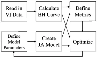
Fig. 2. Automatic magnetic material analysis software structure.
calculate the flux and field strength was done in software after being transferred to a PC.
A toroid was used as the core type to remove the effect of any air gaps and wound with the number of turns to achieve saturation with the driving circuit of the signal generator. The core used in these tests was a Philips TN10/6/4 toroid made of 3F3. The number of turns on the primary and secondary were set to 40 and the primary current monitor resistance was set to 10 . The signal generator frequency was set to 1 kHz and the amplitude varied from approximately 1.2 to 10 Vpp.
The field strength was calculated from the voltage measured across the primary sense resistor using the expression (1) as the field strength is proportional to the applied current in the
pri-mary winding ( )
(1)
The flux density is derived from the voltage on the secondary winding using expression (2). The integration was carried out numerically using trapezoidal integration of the voltage on the secondary winding ( )
(2)
Both the field strength and the flux density were automati-cally calculated in software from the oscilloscope waveforms and after they were transferred to the PC for post-processing.
The overall structure of the analysis software developed is shown in Fig. 2. The software derives the measured field strength ( ) and flux density ( ) from the oscilloscope data, with the test configuration able to be customized. The Jiles–Atherton model can be calculated using the derived field strength from the measured data or an ideal internally generated test waveform (sinusoidal or triangle) and then compared with the original test results. Metrics can be applied to both the measured and simulated results to assess the relative performance of the model, and an optimization loop allows the model parameters to be modified using iteration to achieve optimum model performance. The optimization method uses a steepest descent type of approach.
[image:2.612.49.279.66.248.2]Fig. 3. B–H curves for 3F3 at peak applied field levels of 35, 70, and 140 At/m.
Fig. 4. Basic magnetic measurement metrics.
high-level signal demonstrates the material driven into strong saturation. These waveforms clearly illustrate the range of re-quired waveshapes any model must provide for accurate simu-lation in a wide variety of applications.
III. METRICS FORMAGNETICMATERIALS
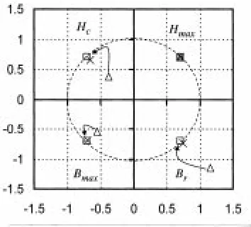
Once the measurements were taken, performance metrics were used to characterize the behavior of the core in a mean-ingful and concise manner. The material’s basic magnetic characteristics can be defined in terms of the fundamental points on the hysteresis curve, which are the maximum field strength ( ) and flux density ( ), the remanence ( ) and the coercive force ( ), all of which are shown in Fig. 4.
Although these metrics are useful, they do not provide a com-plete set for optimization. Fig. 3 shows one such situation, where the material has saturated to such an extent at high field strengths that the hysteresis loop “closes up” prior to the maximum ap-plied field strength being reached. This “early closure” of the loops requires a new parameter to be defined, which is the ap-plied field at which early closure takes place ( ). The mea-surement of where the loop has effectively closed requires the specification of the loop being closed (e.g., to within 1%).
The permeability of the material is also a significant param-eter, and there are two key metrics which can be extracted from
Fig. 5. Basic metric chart with normalization.
the – data. These are the initial permeability and the max-imum incremental permeability at on the – loop.
The area enclosed by the – loop defines the energy loss of the material, and a measurement of this is crucial if temper-ature effects are to be included dynamically in the model. The shape of the loop is also important, as can be seen from the vari-ation in shape of the waveforms in Fig. 3. As the field strength increases, the slope of the hysteresis loop as a whole changes, and the shape changes from an almost elliptical minor loop to the sigmoid shape of saturation.
For electrical circuit simulation, it is important to ensure that the magnetic component parameters chosen result in the correct electrical behavior at the terminals of the device. The metrics can be used to ensure that the model parameters are optimized so that the electrical behavior is accurately represented by the mag-netic component. This may be achieved by including specific electrical metrics such as the response of the magnetic compo-nent to an applied voltage waveform as well as the purely mag-netic metrics. This can be applied in the optimization approach by using the voltage and current waveforms as the goal rather than the – curve.
The chosen set of metrics was extracted from the measured data and the same set of metrics was extracted from the results of simulation. Optimization of the model parameters was achieved by minimizing the difference between either the two sets of met-rics or the least squares error (LSE).
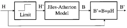
[image:3.612.52.280.256.428.2]Fig. 6. Modified Jiles–Atherton model structure.
IV. MODELING THEMAGNETICMATERIAL
The magnetic material was modeled using PSPICE, although the techniques are generally applicable for most circuit or system simulators. The magnetic model used for the hysteresis characteristic was a modified form of the Jiles–Atherton approach. The original Jiles–Atherton model provides a good model, in general, for sigmoid form hysteresis loops of the form shown in Fig. 3 (the midrange hysteresis measured data). Unfortunately, the model does not handle the problem of early closure as shown in the higher field strength levels, as shown previously in Fig. 3.
The model was therefore modified with two extra parameters. The applied field strength level was limited by the value of at the early closure value ( ). A hard limit function on the applied field was added, modifying this to allow a small slope (ecrate) after limit to avoid complete loop closure and to reduce the discontinuity at the transition to the early closure region. With the limit in place, the model now correctly modeled the early closure, but the slope of the function after closure was too flat. A function was therefore added to the final equation for the flux density ( ) to allow the slope to be varied to give a more realistic hysteresis loop. The structure of the modified model is shown in Fig. 6.
The difficulty with simply changing the slope from a practical simulation point of view is that a discontinuity is introduced to the first derivative of the effective field strength. The function was therefore modified to have a softer limit by changing the linear change to an exponential change of the form given in (3), when the applied field is greater than the early closure field
. (3) While (3) is not continuous in the first derivative generally, if (4) is used to define the value of , then the function becomes continuous through the early closure transitions
ecrate (4)
V. OPTIMIZATION OF THEMODEL TOMEASUREDRESULTS
[image:4.612.325.529.62.211.2]An optimization engine was built into the analysis software to allow optimization of the – hysteresis loop using a LSE cal-culation or minimizing the error between the measured and sim-ulated metrics. The optimization engine has univariate search, simulated annealing, and a genetic algorithm method imple-mented, but the univariate method was applied in this paper.
Fig. 7. Minor loop optimization results.
The optimizer allows the specification of the breadth and depth parameters in a univariate search method, so different types of optimization approach could be implemented. With a breadth type search the parameters are varied, but each parameter has a low number of iterations before moving onto the next param-eter. The breadth type search allows local minima to be gener-ally avoided by searching widely across the solution area. The depth first search allows each parameter to be tuned in turn to the best advantage and is useful where optimization is nearly converged. The optimizer also allows the specification of which parameters are to be allowed to vary, therefore allowing control to be anywhere from completely manual (varying one parameter at a time) to automatic (varying every parameter). The optimizer also allows variable step sizes to ensure that different parameter sensitivities are catered for in the software.
The optimizer was run on the experimental data given in Fig. 2 for 3F3 with the original Jiles–Atherton model and the modified Jiles–Atherton model. The number of outer iterations (breadth) was set to 20 and the number of inner iterations (depth) was set to 5. The LSE calculation was started after the initial magnetization of the model had taken place and a fourth-order Runga–Kutta Integration method was used to calculate the Jiles–Atherton model.
A. Minor Loop (35 At/m) Optimization Results
The 35-At/m field strength measured data was opti-mized using the defined parameters and with the original Jiles–Atherton Model obtained a LSE of 1.8 mT. This corre-sponds to an rms error of 3.8 mT over the range of the – curve. When the modified Jiles–Atherton model was used for the optimization, with the same parameters a LSE of 1.5 mT was reached (rms error of 3.4 mT). The resulting measured and simulated (for the modified model) – curves are shown in Fig. 7.
B. Medium Field Strength (70 At/m) Optimization Results
[image:4.612.55.273.65.113.2]Fig. 8. 70 At/m field strength results.
Fig. 9. Major loop optimization results.
first half cycle as the model goes through the initial magnetiza-tion sequence, but subsequent cycles show a good correlamagnetiza-tion.
C. Major Loop (140 At/m) Optimization Results
The 140-At/m field strength measured data was opti-mized using the defined parameters and with the original Jiles–Atherton Model obtained a LSE of 381 mT. This corre-sponds to an rms error of 17.4 mT over the range of the – curve. When the modified Jiles–Atherton model was used for the optimization, with the same parameters a LSE of 246 mT was reached (rms error of 14.0 mT). The resulting measured and simulated (for the modified model) – curves are shown in Fig. 9.
D. Summary of the Optimized Model Parameters
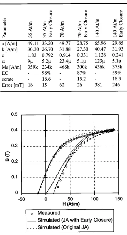
The result of the optimization process with and without the early closure modification are summarized in Table I. The final parameter values after optimization are given and also the error squared for each case. Fig. 10 shows the difference in result when the model is applied with and without the early closure modification for the 140-At/m field strength loop. It can be clearly seen that the loop tips are modeled more accurately using the modified model.
These results indicate that while the Jiles–Atherton model can achieve a good fit to measured data, with or without modifi-cations, there are still considerable variations in the parameter
Fig. 10. Comparison of the original and modified Jiles–Atherton model loops.
values derived across the range of operation of the model from minor to major loops.
E. Proposed Modification to the Optimization Goal Function
It is the view of the authors that although the LSE function is the best general method for optimizing curves of this kind, it is often essential to ensure that a particular facet of the – loop characteristic is modeled extremely accurately. This leads to the use of the previously defined metrics as a method of ensuring that specific features of the behavior are optimized for directly, instead of the more general least squares approach.
To implement this in software requires a simple modification to the error calculation so that instead of calculating the error using least squares, the error is the normalized deviation from the defined metrics, with appropriate weighting factors for each metric. This is defined in (5)
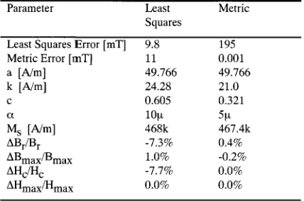
[image:5.612.66.265.247.399.2]TABLE II
COMPARISON OFLEASTSQUARES ANDMETRICOPTIMIZATION
where
metric of the simulated curve; metric of the measured curve; individual weighting for the metric.
The advantage of this method is that the optimization of the material characteristic can be tailored for the end application. For example, a communications pulse transformer may need ex-cellent modeling of the minor loop slope, whereas a power trans-former may need more emphasis on the area of the – loop for energy calculations. The error function for different applica-tions can be easily defined using the weighting factors in (5). For example, in the characterization of the 3F3 material thus far in this paper, the method used has been a least squares approach. If the metrics previously defined are applied for an optimiza-tion run of a major loop with a LSE of 0.098 T (rms error of 8.85 mT) then although the error is quite small for the whole curve, the normalized error for the remanence is 7.2% and the normalized error for the coercive force is 7.7%.
When the optimization is repeated, but this time using the goal function defined by the remanence, coercive force and maximum and , the LSE increases to 0.195 T (rms error of 12.49 mT) but the normalized error for the remanence reduced to 0.4% and the coercive force reduced to 0%. The normalized errors on the maximum reduced from 0.9% to 0.17%. The full set of model parameters after optimization and the relative errors are given in Table II.
The – curves for the metric and least squares opti-mized parameters are shown in Fig. 11 (using the modified Jiles–Atherton model). It can be seen that although the resulting curves are similar, the metric optimized – curves have improved accuracy at the key crossing points and .
F. Notes on the Optimization Procedure
[image:6.612.57.271.95.237.2]The optimization of the – curves at different field strengths, as summarized in Table I, clearly shows the diffi-culty in assigning a single parameter set to the Jiles–Atherton model for all values of field strength. There are significant differences in the optimized parameters highlighted between minor and major loops, and Lederer et al. [7] have addressed this problem by setting the values of and to fixed values and tightly constraining the values of and during the
Fig. 11. Comparison of metric and least squares optimizedB–H curves.
optimization process. This does reduce the risk of convergence to a poor solution in the optimization process, but does not necessarily give the flexibility to achieve an excellent fit of the – curve. Carpenter [8] has proposed a modification to the Jiles–Atherton model to address the issue of minor loops, and this approach has been implemented by Dallago et al. [9] for the modeling of high frequency transformers. This approach would certainly provide an improvement in the generality of parameters and could be easily implemented as the core model in the optimization method.
The comparison in Table II of the two goal functions used in the optimization procedure and the resulting – curves indi-cate that, in general, the least squares approach gives a good ap-proximation to the overall shape of the – curve under test, but that the metric approach gives an near exact match of the key features of the model. This allows the designer to select the optimization method to achieve the match that is required for the application. It is also clear that the least squares fit can be considered as another metric, and could simply be added to the list of metrics used by the optimizer. This would allow the mag-netics designer to trade off the exact fitting of key features with the best fit of the overall – curve shape.
VI. SUMMARY
This paper has presented methods for optimizing models of magnetic materials using the Jiles–Atherton approach, investigating the issue of characterizing materials and applying metrics.
Modifications to the Jiles–Atherton model for the accurate representation of the early closure effect when heavily saturated have been presented and a resulting improvement demonstrated in the optimization of the model parameters.
dressed and a possible solution presented. Comparable opti-mization simulations have shown a significant improvement in accuracy by adding these extensions to the model. The specific problems of early closure and slope changes in the – loop have been addressed using a modified Jiles–Atherton approach. The optimization of the – loop for a range of loops from small minor to heavily saturated major has highlighted the problem with the original Jiles–Atherton model in im-plementing a general purpose model which can accurately represent the material over a wide range of operation. This is clearly demonstrated in Table I, where the parameter values for particular levels vary widely.
The problem of how to assess the quality of an optimized model using metrics shows how using different goal functions can guide the optimizer intelligently to a solution that is appro-priate for the application in question. A goal function was pre-sented which will allow this to take place and was demonstrated to give better optimization results for specific parameters of the
– curve than a generic least squares approach.
Using a modified Jiles–Atherton model and specific metrics to characterize the model parameters, much greater accuracy in the eventual circuit simulation can be achieved. Using a mod-ified Jiles–Atherton model and specific metrics to characterize the model parameters, much greater accuracy in the eventual cir-cuit simulation can be achieved. The advantage of this approach is that the model parameters are tailored to meet the needs of the particular application. For an ADSL transformer, the model could be optimized to ensure high accuracy of minor loops and hence the operating distortion could be estimated using simu-lation to a much higher accuracy than obtained using a least squares optimized model. For a power supply transformer, the resulting model could be optimized to ensure that the area of the loop, and hence the power dissipated was correct, thus ensuring that the circuit simulation could provide much better estimates of power loss and efficiency.
REFERENCES
[1] D. C. Jiles and D. L. Atherton, “Ferromagnetic hysteresis,” IEEE Trans.
Magn., vol. MAG-19, pp. 2183–2185, Sept. 1983.
teresis loops of soft magnetic materials,” IEEE Trans. Magn., vol. 32, pp. 489–496, Mar. 1996.
[7] D. Lederer, H. Igarashi, A. Kost, and T. Honma, “On the parameter iden-tification and application of the Jiles–Atherton hysteresis model for nu-merical modeling of measured characteristics,” IEEE Trans. Magn., vol. 35, pp. 1211–1214, May 1999.
[8] K. H. Carpenter, “A differential equation approach to minor loops in the Jiles–Atherton hysteresis model,” IEEE Trans. Magn., vol. 27, pp. 4404–4406, Nov. 1991.
[9] E. Dallago, G. Sassone, and G. Venchi, “High frequency power trans-former model for circuit simulation,” IEEE Trans. Power Electron., vol. 12, pp. 664–670, July 1997.
Peter R. Wilson (M’98–S’99) received the B.Eng. degree in electrical and
elec-tronic engineering, the Postgraduate Diploma in digital systems engineering, and the M.B.A degree, all from Heriot-Watt University, in 1988, 1992, and 1999, respectively.
He worked in the Navigation Systems Division of Ferranti plc, Edinburgh, Scotland from 1988 to 1990 on Fire Control Computer systems, before moving in 1990 to the Radar Systems Division of GEC-Marconi Avionics, also in Ed-inburgh. From 1990 to 1994, he worked on modeling and simulation of power supplies, signal processing systems, servo, and mixed technology systems. From 1994 to 1999, he worked as European Product Specialist with Analogy Europe, Swindon, U.K. During that time, he developed a number of models, libraries, and modeling tools for the Saber simulator, especially in the areas of power systems, magnetics, and telecommunications. Since 1999, he has been working toward the Ph.D. degree at the University of Southampton, U.K. His current re-search interests include modeling of magnetic components in electric circuits, VHDL-AMS modeling and simulation, and the development of electronic de-sign tools.
Mr. Wilson is a Member of the Institute of Electrical Engineers and a Char-tered Engineer.
J. Neil Ross received the B.Sc. degree in physics in 1970 and the Ph.D. degree
in 1974 for work on the physics of ion laser discharges, both from the University of St. Andrews.