http://dx.doi.org/10.4236/ns.2011.32021
Two solutions for the BVP of a rotating
variable-thickness solid disk
Ashraf M. Zenkour1,2, Suzan A. Al-Ahmadi1
1Department of Mathematics, Faculty of Science, King AbdulAziz University, Jeddah, Saudi Arabia; Coresponding Author:
2Department of Mathematics, Faculty of Science, Kafr El-Sheikh University, Kafr El-Sheikh, Egypt;
Received 23 November 2010; revised 25 December 2010; accepted 28 December 2010.
ABSTRACT
This paper presents the analytical and numeri-cal solutions for a rotating variable-thickness solid disk. The outer edge of the solid disk is considered to have free boundary conditions. The governing equation is derived from the ba-sic equations of the rotating solid disk and it is solved analytically or numerically using finite difference algorithm. Both analytical and nu-merical results for the distributions of stress function and stresses of variable-thickness solid disks are obtained. Finally, the distributions of stress function and stresses are presented and the appropriate comparisons and discussions are made at the same angular velocity.
Keywords:Rotating, Solid Disk, Variable Thickness, Analytical Method, Finite Difference Method
1. INTRODUCTION
The theoretical and experimental investigations on the rotating solid disks have been widespread attention due to the great practical importance in mechanical engi-neering. Rotating disks have received a great deal of attention because of their widely used in many me-chanical and electronic devices. They have extensive practical engineering application such as in steam and gas turbines, turbo generators, flywheel of internal com- bustion engines, turbojet engines, reciprocating engines, centrifugal compressors and brake disks. The problems of rotating solid disks have been performed under vari-ous interesting assumptions and the topic can be easily found in most of the standard elasticity books [1,2]. For a better utilization of the material, it is necessary to al-low variation of the effective material or thickness prop-erties in one direction of the solid disk.
The problems of rotating variable-thickness solid disks
are rare in the literature. Most of the research works are concentrated on the analytical solutions of rotating iso-tropic disks with simple cross-section geometries of uniform thickness and specifically variable thickness. The solution of a rotating solid disk with constant thick-ness is obtained by Gamer [3,4] taking into account the linear strain hardening material behavior. The inelastic and viscoelastic deformations of rotating variable- thickness solid disks have been presented in the litera-ture [5-8]. Eraslan [5], and Eraslan and Orcan [6] have analytically studied rotating disks of exponentially varying thickness and of linearly strain hardening mate-rial. Eraslan [7] has presented the stress distributions in elastic-plastic rotating disks with elliptical thickness pro- files using Tresca and von Mises criteria. Zenkour and Allam [8] have developed analytical solution for the analysis of deformation and stresses in elastic rotating viscoelastic solid and annular disks with arbitrary cross- sections of continuously variable thickness.
As many rotating components in use have complex cross-sectional geometries, they cannot be dealt with using the existing analytical methods. Numerical meth-ods, such as the finite element method [9], the boundary element method [10] and Runge-Kutta’s algorithm [11], can be applied to cope with these rotating components.
You et al. [11] have numerically studied rotating solid
disks of uniform thickness and constant density as well as annular disks of variable thickness and variable den-sity. In a recent paper, Zenkour and Mashat [12] have presented both analytical and numerical solutions for the analysis of deformation and stresses in elastic rotating disks with arbitrary cross-sections of continuously vari-able thickness.
(FDM) is also introduced to solve the governing equa-tion. A comparison between both analytical and numeri-cal solutions is made. Finally, a number of application examples are given to demonstrate the validity of the proposed method.
2. BASIC EQUATIONS
As the effect of thickness variation of rotating solid disks can be taken into account in their equation of mo-tion, the theory of the variable-thickness solid disks can give good results as that of uniform-thickness disks as long as they meet the assumption of plane stress. The present solid disk is considered as a single layer of vari-able thickness. After considering this effect, the equation of motion of rotating disks with variable thickness can be written as
2 2d 0,
dr hrr hh r (1)
where r and are the radial and circumferential
stresses, h is the variable thickness of the disk, r is the radial coordinate, is the material density of the ro-tating solid disk and is the constant angular velocity.
The relations between the radial displacement u and the strain components are irrespective of the thickness of the rotating solid disk. They can be written as
d
, ,
d
r
u u
r r
(2) where r and are the radial and circumferential
strains, respectively. The above geometric relations lead to the following condition of deformation harmony:
d
0.
dr r r (3)
For the elastic deformation, the constitutive equations for the variable-thickness solid disk can be described with Hooke’s law
, ,
r r
r
E E
(4) where E is Young’s modulus and is Poisson’s ratio. Introducing the stress function and assuming that the following relations hold between the stresses and the stress function
2 2
1 d
, .
d
r r
hr h r
(5) Substituting Eq.5 into Eq.4, one obtains
2 2
2 2
1 1 d ,
d
1 1 d
. d
r E hr h r r
r E h r hr
(6)
3. FORMULATION AND ANALYTIC
ELASTIC SOLUTION
The substitution of Eq.6 into Eq.3 produces the fol-lowing confluent hypergeometric differential equation for the stress function ( ) :r
2 2
2
2 3
d d d
1
d d
d d
1 3 0.
d
r h
r r
h r r r
r h h r
h r
(7)
The boundary conditions for the rotating solid disk are at 0,
0 at .
r r
r r b
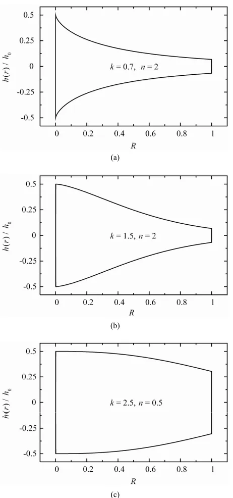
(8) The thickness of the solid disk is assumed to vary nonlinearly through the radial direction. It is assumed to be in terms of a simple exponential power law distribu-tion according to the following case:
0e ,k r n
b
h r h
(9) where h0 is the thickness at the middle of the disk, n
and k are geometric parameters and b is the outer radius of the disk (see Figure 1). The value of n equal to zero represents a uniform-thickness solid disk while the value of k equal to unity represents a linearly decreasing vari-able-thickness solid disk. For small k and large n (k = 0.7 or 1.5 and n = 2) the profile of the solid disk is concave while it is convex for large k and small n (k = 2.5 and n = 0.5). It is to be noted that the parameter n determines the thickness at the outer edge of the solid disk relative to
0
h while the parameter k determine the shape of the profile.
Introducing the following dimensionless forms:
2 0
1 2 2
1 2 2
/
3 ,
1
,
, , ,
1
, , .
r
r
R r b b
R r
bh E
(10)
Then, Eq.7 may be written in the following simple form
2
2 3
2
d d
1 1 e 0.
d d
k
k k nR
R knR R kn R R
R
R
(a)
(b)
[image:3.595.57.288.80.573.2](c)
Figure 1. Variable-thickness solid disk profiles for (a) k = 0.7 and n = 2, (b) k = 1.5 and n = 2 and (c) k = 2.5 and n = 0.5.
written as
2 2
, 1 ,
, 2 ,
e d
d ,
k
k nR R
i j i j
R
i j i j
R R M R C F W
W R C F M
(12) where C1 and C2 are arbitrary constants, is a
dummy parameter, Mi j, and Wi j, are Whittaker’s
functions
, , , , , , , ,
k k
i j i j
M R M i j nR W R W i j nR (13)
in which
1 1
, , 0.
2
i j k
k k
(14) In addition, the function F R
is given in terms of Whittaker’s functions by
2 2 2
, 1, , 1,
e
. 1
k k nR
i j i j i j i j
R F R
W R M R kM R W R
(15) The substitution of Eq.12 into Eq.5 with the aid of the dimensionless forms given in Eq.10 gives the radial and circumferential stresses in the following forms:
2 1 2
1 , 1 ,
, 2 ,
e d
d ,
k
k nR R
i j i j
R
i j i j
R R M R C F W
W R C F M
(16)
22
d
e .
d 3
k
nR R
R
R
(17)
Here, the first derivative of the stress function
R with respect to R may be given easily by using Eq.12. Note that the first derivatives of Whittaker’s functions,
i j
M and Wi j, can be represented by
1
, 2 ,
1
1, 2
1
, 2 , 1,
d d
,
d .
d
k
i j i j
i j k
i j i j i j
k
M R nR i M R
R R
i j M R
k
W R nR i W R W R
R R
(18)
Finally, the stress function
R and consequently the stresses 1
R and 2
R may be determined completely after applied the dimensionless of the boundary conditions given in Eq.8.4. FINITE DIFFERENCE ALGORITHM
The resolution of the elastic problem of rotating solid disk with variable thickness is to solve a second-order differential equation, Eq.11, under the given boundary conditions
0
1 0 such that 1
0 2
0 . Eq.11 can be written in the following general form:
,p R q R s R
2
1 ,
1 ,
e k .
k
k
nR knR p R
R kn R q R
R
s R R
(20)
It is clear that the above problem has a unique solution because p R q R
, , and s R
are continuous on [0,1] and q R
0 on [0,1]. The linear second-order boundary value problem given in Eq.19 requires that difference-quotient approximations be used for ap-proximating and . First we select an integer0
N and divided the interval [0,1] into
N1
equal subintervals, whose end points are the mesh points,
i
R i R for i0,1,...,N1, where R 1/
N1
. At the interior mesh points, Ri, i1, 2,..., ,N the dif-ferential equation to the approximated is
.
Ri p Ri Ri q Ri Ri s Ri (21) If we apply the centered difference approximations of
Ri and
Ri to Eq.21, we arrive at the system(see Eq.22):
for each i1, 2,..., .N The N equations, together with the boundary conditions
0
1
0, 0,
N
(23) are sufficient to determine the unknowns i,
0,1, 2,..., 1
i N . The resulting system of Eq.22 is ex-presses in the tri-diagonal N N -matrix form:
,
A B (24) where
2 ,
, 1
, 1
, , 2
2 ( ) ( ), 1, 2,..., , 1 ( ), 1, 2,..., 1,
2
1 ( ), 2,3,..., , 2
0, 1, 2,..., 2, 3, 4,..., , 2, ( ) ( ), 1, 2,..., .
i i i
i i i
i i i
i j j i
i i
A R q R i N
R
A p R i N
R
A p R i N
A A i N j N j i
B R s R i N
(25) The solution of the finite difference discretization of the two-point linear boundary value problem can there-fore be found easily even for very small mesh sizes.
5. NUMERICAL EXAMPLES AND
DISCUSSION
Some numerical examples for the rotating variable- thickness solid disks will be given according the ana-lytical and numerical solutions
0.3
. According to Eq.10, the stress function , the radial stress 1 andthe circumferential stress 2 determined as per the
analytical solution are compared with those obtained by the numerical FDM solution.
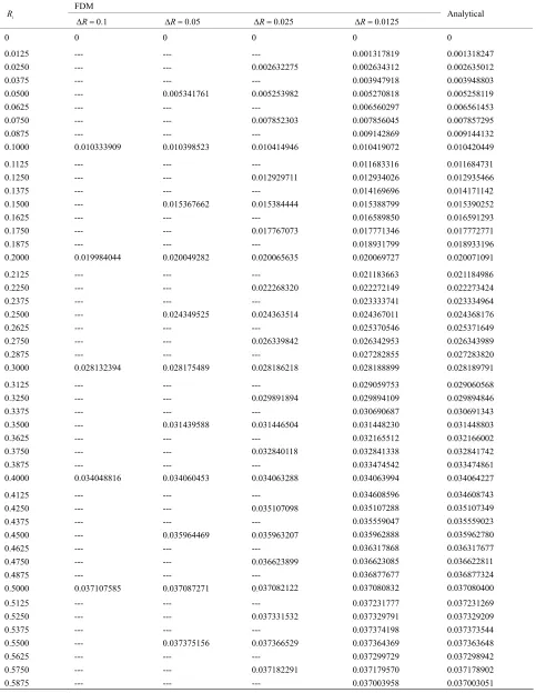
The results of the present investigations for the stress function are reported in Table 1 for rotating vari-able-thickness solid disk with k = 2.5 and n = 0.5. For this example, N = 9, 19, 39 and 79, so R has the cor-responding values 0.1, 0.05, 0.025 and 0.0125, respec-tively. The FDM gives results compared well with the exact solution, especially for small values of R. The relative error between the exact method and the FDM with R 0.0125, may be less than 1.3 10 4.
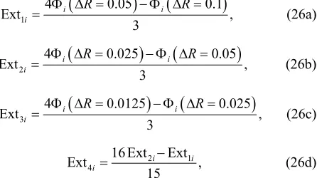
Richardson’s extrapolation method is applied here with R 0.1,0.05,0.025, and 0.0125 and the obtained results are listed in Table 2. These extrapolations are given, respectively by
1
4 0.05 0.1
Ext ,
3
i i
i
R R
(26a)
2
4 0.025 0.05
Ext ,
3
i i
i
R R
(26b)
3
4 0.0125 0.025
Ext ,
3
i i
i
R R
(26c)
2 1 4
16 Ext Ext
Ext ,
15
i i
i
[image:4.595.316.539.360.485.2] (26d)
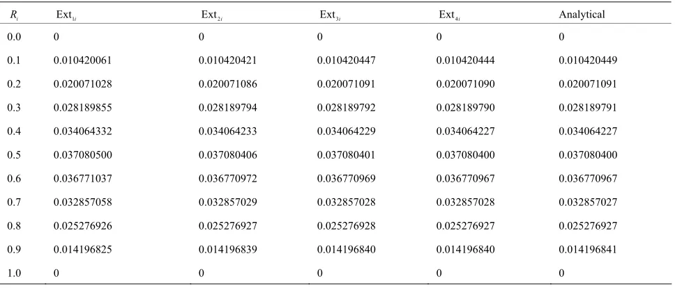
Table 2 shows that all extrapolations results are cor-rect to the decimal places listed. In fact, if sufficient dig-its are maintained, the approximation of Ext4i gives
results those agree with the exact solution with maxi-mum difference error of 1.0 10 9 at some of the mesh
points. Additional results for the stress function are reported for rotating variable-thickness solid disk with k
= 0.7 and n = 2 in Table 3 and with k = 1.5 and n = 2 in
Table 4. Once again, the FDM gives results compared
well with the exact analytical solution, especially for small values of R.
Now the least square method and curve fitting are used for the discrete results of the stress function . So, one can get easily the radial and circumferential stresses
2
21 1
1 2 1 ,
2 i i i i 2 i i i
R p R R q R Rp R R s R
Table 1. Dimensionless stress function of a rotating variable-thickness solid disk (k = 2.5, n = 0.5). FDM i R 0.1 R
0.05 R 0.025 R 0.0125 R Analytical
0 0 0 0 0 0
0.6000 0.036832186 0.036786324 0.036774810 0.036771929 0.036770967 0.6125
0.6250 0.6375 0.6500 0.6625 0.6750 0.6875 0.7000
--- --- --- --- --- --- ---
0.032936503
--- --- ---
0.035291940 ---
--- ---
0.032876919
---
0.036140911 ---
0.035278284 ---
0.034185494 ---
0.032862001
0.036483294 0.036137738 0.035734998 0.035274868 0.034757198 0.034181892 0.033548911 0.032858271
0.036482282 0.036136679 0.035733896 0.035273729 0.034756025 0.034180690 0.033547685 0.032857027 0.7125
0.7250 0.7375 0.7500 0.7625 0.7750 0.7875 0.8000
--- --- --- --- --- --- ---
0.025353741
--- --- ---
0.029540441 ---
--- ---
0.025296129
---
0.031308165 ---
0.029525248 ---
0.027515416 ---
0.025281728
0.032110047 0.031304368 0.030441421 0.029521449 0.028544751 0.027511682 0.026422653 0.025278128
0.032108789 0.031303102 0.030440152 0.029520183 0.028543493 0.027510437 0.026421427 0.025276927 0.8125
0.8250 0.8375 0.8500 0.8625 0.8750 0.8875 0.9000
--- --- --- --- --- --- ---
0.014247568
--- --- ---
0.020171897 ---
--- ---
0.014209433
---
0.022828123 ---
0.020159404 ---
0.017281209 ---
0.014199988
0.024078628 0.022824727 0.021517051 0.020156281 0.018743148 0.017278432 0.015762966 0.014197627
0.024077458 0.022823594 0.021515961 0.020155240 0.018742161 0.017277507 0.015762106 0.014196841 0.9125
0.9250 0.9375 0.9500 0.9625 0.9750 0.9875 1.0000
--- --- --- --- --- --- --- 0
--- --- ---
0.007463350 ---
--- --- 0
---
0.010922960 ---
0.007458083 ---
0.003814000 ---
0
0.012583344 0.010921087 0.009211874 0.007456766 0.005656864 0.003813309 0.001927282 0
[image:6.595.57.541.517.724.2]0.012582635 0.010920462 0.009211340 0.007456327 0.005656526 0.003813078 0.001927164 0
Table 2. Dimensionless stress function of a rotating variable-thickness solid disk using Richardson’s extrapolation method with different values of ΔR (k = 2.5, n = 0.5).
i
R Ext1i Ext2i Ext3i Ext4i Analytical
0.0 0 0 0 0 0
0.1 0.010420061 0.010420421 0.010420447 0.010420444 0.010420449
0.2 0.020071028 0.020071086 0.020071091 0.020071090 0.020071091
0.3 0.028189855 0.028189794 0.028189792 0.028189790 0.028189791
0.4 0.034064332 0.034064233 0.034064229 0.034064227 0.034064227
0.5 0.037080500 0.037080406 0.037080401 0.037080400 0.037080400
0.6 0.036771037 0.036770972 0.036770969 0.036770967 0.036770967
0.7 0.032857058 0.032857029 0.032857028 0.032857028 0.032857027
0.8 0.025276926 0.025276927 0.025276928 0.025276927 0.025276927
0.9 0.014196825 0.014196839 0.014196840 0.014196840 0.014196841
Table 3. Dimensionless stress function of a rotating variable-thickness solid disk (k = 0.7, n = 2).
FDM
Analytical 0.0125
R
0.025
R
0.05
R
0.1
R
i
R
0 0
0 0
0 0.0
0.003891568 0.003891627
0.003891774 0.003892229
0.003893631 0.1
0.006897877 0.006898133
0.006898890 0.006901872
0.006913732 0.2
0.008971625 0.008972022
0.008973209 0.008977938
0.008996897 0.3
0.010102762 0.010103227
0.010104619 0.010110178
0.010132490 0.4
0.010321685 0.010322155
0.010323563 0.010329193
0.010351793 0.5
0.009683519 0.009683947
0.009685228 0.009690352
0.009710919 0.6
0.008256930 0.008257280
0.008258329 0.008262527
0.008279371 0.7
0.006116796 0.006117044
0.006117787 0.006120761
0.006132695 0.8
0.003339509 0.003339638
0.003340026 0.003341577
0.003347797 0.9
0 0
0 0
[image:7.595.56.538.350.566.2]0 1.0
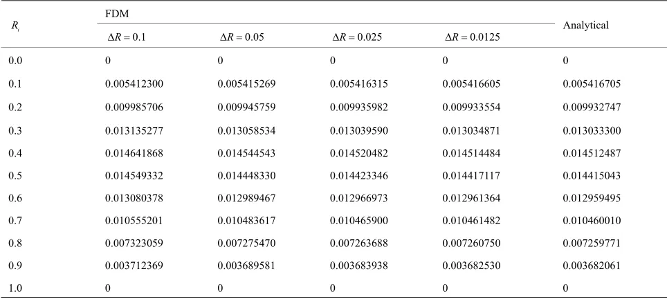
Table 4. Dimensionless stress function of a rotating variable-thickness solid disk (k = 1.5, n = 2).
FDM
Analytical 0.0125
R
0.025
R
0.05
R
0.1
R
i
R
0 0
0 0
0 0.0
0.005416705 0.005416605
0.005416315 0.005415269
0.005412300 0.1
0.009932747 0.009933554
0.009935982 0.009945759
0.009985706 0.2
0.013033300 0.013034871
0.013039590 0.013058534
0.013135277 0.3
0.014512487 0.014514484
0.014520482 0.014544543
0.014641868 0.4
0.014415043 0.014417117
0.014423346 0.014448330
0.014549332 0.5
0.012959495 0.012961364
0.012966973 0.012989467
0.013080378 0.6
0.010460010 0.010461482
0.010465900 0.010483617
0.010555201 0.7
0.007259771 0.007260750
0.007263688 0.007275470
0.007323059 0.8
0.003682061 0.003682530
0.003683938 0.003689581
0.003712369 0.9
0 0
0 0
0 1.0
since we have as a continuous function of R. The distributions of the stress function, radial and circum-ferential stresses are presented in Figure 2. The numeri-cal FDM solution is compared with the exact analytinumeri-cal solution for the rotating variable-thickness solid disk with k = 2.5 and n = 0.5. It can be seen that the FDM can describe the stress function and stresses through the thickness of the rotating solid disk very well enough.
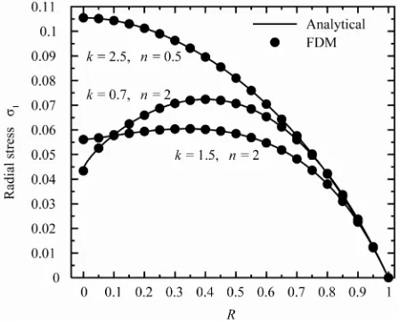
For the sake of completeness and accuracy, additional results for the stress function and stresses are presented in Figures 3-5 for different values of the geometric pa-rameters k and n. Figure 3 shows the stress function
through the radial direction of the rotating solid disk with k = 2.5, n = 0.5; k = 0.7, n = 2 and k = 1.5, n = 2. Similar results for the radial 1 and the circumferential
2
stresses are plotted in Figures 4 and 5. Figure 3 shows that the stress function increases as k in-creases and this irrespective of the value of n (see also Tables 3 and 4). Figures 4 and 5 show that k = 2.5, n = 0.5 gives the largest stresses. The intersection of the two cases k = 0.7, n = 2 and k = 1.5, n = 2 may be occurred at
R = 0.1 for the radial stress and at R = 0.15 for the circumferential stress.
Figure 2. Stress function Ф, radial stress σ1 and
circumferen-tial stress σ2 for the variable-thickness solid disk.
[image:8.595.311.535.79.259.2]Figure 3. Stress function Ф of the variable-thickness solid disk for different values of k and n.
Figure 4. Radial stress σ1 of the variable-thickness solid disk
[image:8.595.59.284.295.468.2]for different values of k and n.
Figure 5. Circumferential stress σ2 of the variable-thick- ness
solid disk for different values of k and n
.
consequently, stresses with excellent accuracy with the exact analytical solution. In most cases of rotating vari-able-thickness solid disks, the analytical solutions are not available. In these cases, one can trustily use the pre-sent FDM solutions.
6. CONCLUSIONS
The rotating solid disk with variable thickness is treated herein. By introducing a suitable stress function, the governing equation is derived from the equation of motion of rotating disk, compatibility equation and the proposed stress-strain relationship. Both the analytical and numerical solutions are presented. The calculation of the rotating solid disk is turned into finding the solution of a second-order differential equation under the given conditions at the center and the outer edge of the disk. The numerical solution is based upon the finite differ-ence method. The governing equation is solved analyti-cally with the help of Whittaker’s functions and a num-ber of numerical examples are studied. The results of the two solutions at different disk configurations are com-pared. The proposed FDM approach gives very agree-able results to the analytical solution and so it may be used for different problems that analytical solutions are not available.
REFERENCES
[1] Timoshenko, S.P. and Goodier, J.N. (1970) Theory of elasticity. McGraw-Hill, New York.
[2] Ugural, S.C. and Fenster, S.K. (1987) Advanced strength and applied elasticity. Elsevier, New York.
[3] Gamer, U. (1984) Elastic-plastic deformation of the ro-tating solid disk. Ingenieur-Archiv, 54, 345-354.
[image:8.595.59.283.513.694.2]elas-tic-plastic disk. ZAMM, 65, T136-137.
[5] Eraslan, A.N. (2000) Inelastic deformation of rotating variable thickness solid disks by Tresca and Von Mises criteria. International Journal of Computational Engi-neering Science,3, 89-101.
[6] Eraslan, A.N. and Orcan, Y. (2002) On the rotating elas-tic-plastic solid disks of variable thickness having con-cave profiles. International Journal of Mechanical Sci-ences, 44, 1445-1466.
[7] Eraslan, A.N. (2005) Stress distributions in elastic-plastic rotating disks with elliptical thickness profiles using Tresca and von Mises criteria. ZAAM,85, 252-266. [8] Zenkour, A.M. and Allam, M.N.M. (2006) On the
rotat-ing fiber-reinforced viscoelastic composite solid and an-nular disks of variable thickness. International Journal
for Computational Methods in Engineering Science, 7,
[9] Zienkiewicz, O.C. (1971) The finite element method in engineering science. McGraw-Hill, London.
[10] Banerjee, P.K. and Butterfield, R. (1981) Boundary ele-ment methods in engineering science. McGraw-Hill, New York.
[11] You, L.H., Tang, Y.Y., Zhang, J.J. and Zheng, C.Y. (2000) Numerical analysis of with elastic-plastic rotating disks arbitrary variable thickness and density. The Interna-tional Journal of Solids and Structures, 37, 7809-7820.
[12] Zenkour, A.M. andMashat, D.S. (2010), Analytical and numerical solutions for a rotating disk of variable thick-ness. Applied Mathematics, 1, 430-437.