ISSN Online: 2152-7393 ISSN Print: 2152-7385
DOI: 10.4236/am.2019.109052 Sep. 18, 2019 728 Applied Mathematics
Analysis of an Inventory System for
Items with Stochastic Demand and
Time Dependent Three-Parameter
Weibull Deterioration Function
Nwoba Pius Ophokenshi
1, Chukwu Walford Ikechukwu Emmanuel
2, Maliki Olaniyi Sadik
31Department of Industrial Mathematics and Applied Statistics, Ebonyi State University, Abakaliki, Nigeria 2Department of Statistics, University of Nigeria, Nsuka, Nigeria
3Department of Mathematics, Michael Okpara University of Agriculture, Umudike, Nigeria
Abstract
In recent times, mathematical models have been developed to describe various scenarios obtainable in the management of inventories. These models usually have as objective the minimizing of inventory costs. In this research work we propose a mathematical model of an inventory system with time-dependent three-parameter Weibull deterioration and a stochastic type demand in the form of a negative exponential distribution. Explicit expressions for the op-timal values of the decision variables are obtained. Numerical examples are provided to illustrate the theoretical development.
Keywords
Inventory Model, Deteriorating Items, Weibull Distribution, Stochastic Demand, MathCAD14
1. Introduction
Inventory holding refers to producing ahead of demand and sales realizations [1]. The total investment in inventories is enormous and accounts for nearly half of the total logistics cost [2]. In view of this high cost, the management of in-ventory offers high potential for improvement and results in a relatively rich li-terature on theoretic inventory models. In inventory planning and control, the performance measures adopted should encourage the positive aspects of holding inventory such as providing flexibility, providing resources for production, pro-viding responsive customer service. We observe that inventory arises in many
How to cite this paper: Ophokenshi, N.P., Emmanuel, C.W.I. and Sadik, M.O. (2019) Analysis of an Inventory System for Items with Stochastic Demand and Time Depen-dent Three-Parameter Weibull Deteriora-tion FuncDeteriora-tion. Applied Mathematics, 10, 728-742.
https://doi.org/10.4236/am.2019.109052
Received: June 11, 2019 Accepted: September 15, 2019 Published: September 18, 2019
Copyright © 2019 by author(s) and Scientific Research Publishing Inc. This work is licensed under the Creative Commons Attribution International License (CC BY 4.0).
http://creativecommons.org/licenses/by/4.0/
DOI: 10.4236/am.2019.109052 729 Applied Mathematics different situations. It is unlikely that the same inventory planning and control considerations will apply equally to all categories of inventory [3].
Some type of products may undergo change in value in storage. They may become partially or entirely unfit for consumption in the course of time. This change or deterioration can be defined as any process that prevents an item from being used for its intended original purpose. Following its utility, the deteriorat-ing item can be characterized into either an item whose functionality or physical fitness deteriorates over time (e.g. fresh food or medicine) or an item whose functionality does not degrade, but where demand deteriorates over time as customers’ perceived utility decreases (e.g. fashion clothes, high technology products or newspapers). Both categories pertain to the same problem but re-quire different actions seeing that items that lose their functional characteris-tics and quality often cannot, or should not be kept in inventory. However, items that lose perceived utility can be kept in inventory and may be sold on a secondary market.
The main objective of inventory management for deteriorating items is to ob-tain optimal returns during the useful lifetime of the product [3]. This leads to three main issues: determining reasonable and appropriate methods for issuing inventory, replenishing inventory and allocating inventory. The choice of in-ventory valuation methods adopted in issuing inin-ventory (i.e. the order in which the items are to be issued), such as methods based on time sequence including FIFO (first-in, first-out) and LIFO (last-in, first-out), depends on both the in-trinsic characteristics of the inventory (e.g. lifetime, quantity, variety, issuing frequency etc.) and the influence on the company (e.g. inventory balance, cost of goods sold etc.) [4].
1.1. Mathematical Formulation
A rich literature on modelling of deteriorating inventory shows how the deteri-oration of products has been captured in the research problem up till now. To integrate deterioration into mathematical models, the model type (deterministic or stochastic) and the considered time horizon (infinite or finite) lead to specific methods [4].
1.2. Deterioration Process Modeling Approaches
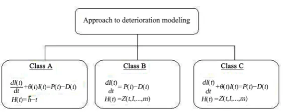
Many researchers have analyzed inventory control of deteriorating items from different perspectives. Broadly speaking, the existing literature in this field can be divided into the following three classes from the perspective of the modeling approach. These classes are schematically illustrated in Figure 1.
( )
I t : On-hand inventory as a function of time t.
( )
tθ : Deterioration function of time t.
( )
D t : Demand function of time t.
( )
P t : Production rate as a function of time t.
( )
DOI: 10.4236/am.2019.109052 730 Applied Mathematics Figure 1.Categorization of deterioration modeling schemes.
h: A positive constant.
(
, , ,)
Z t I m : A non-linear increasing positive function of finite number of
parameters such as stocking time, t, on-hand inventory, I, etc.
1.2.1. Class A: Non-Linear Inventory Function
Most researches on deteriorating inventory consider that inventory decays with time, in different patterns. Thus, the on-hand inventory function can be deter-mined by the differential equation:
( )
( ) ( )
( )
( )
d
d I t
t I t P t D t
t +
θ
= − (1)here I t
( )
is the inventory level at time t, P t( )
and D t( )
indicate thedete-rioration rate functions, the production rate and the demand rate as a function of time t respectively
In this type of research it is considered that the holding cost per unit item per unit time (holding cost rate) is constant. In other words, the holding cost is li-near in terms of parameters like stocking time, t, and the on-hand inventory lev-el, I, that can be stated as htI , h>0 where is constant.
This kind of modeling approach is more appropriate for decaying items and was used in the earliest researches on deteriorating products. Ghare and Schrad-er [5]seem to have been the first to have developed an exponentially deteriorat-ing inventory model by defindeteriorat-ing a constant decaydeteriorat-ing rate.
1.2.2. Class B: Non-Linear Holding Cost
The deterioration process directly affects the on-hand inventory function and thereby inventory holding cost modeling. In this category, the on-hand invento-ry function form is similar to its form of non-deteriorating products and can be obtained by the differential equation:
( )
( )
( )
d d I t
P t D t
t = − (2)
Here, instead of considering the deterioration rate function, θ
( )
t in theon-hand inventory function, the holding cost, H, is considered as a non-linear increasing positive function of parameters like stocking time, t or on-hand in-ventory I.
DOI: 10.4236/am.2019.109052 731 Applied Mathematics deteriorating items-especially perishable ones—when the value and quality of the unsold items decrease with time, as in the case of green vegetables. For products such as electronic components, radioactive substances, volatile liquids etc., where more sophisticated tools are required for their security and safety in stock, a non-linear stock-dependent holding cost can be appropriate.
1.2.3. Class C: Non-Linear Inventory Function and Non-Linear Holding Cost
This modeling approach is more complicated than the other two. Here, both the deterioration rate function, θ
( )
t , a feature of Class A, and the non-linearhold-ing cost, a feature of Class B, are considered to model the inventory system of deteriorating products. In [6] the authors discussed Goh’smodel, considering a constant θ
( )
t in addition to non-linear holding cost in two time-dependentand stock-dependent cases.
1.3. The Demand Characteristics
The customer arrival rate per time period may be deterministic or stochastic, each individual demand may be deterministic or stochastic and each individual demand may also be discrete or continuous [7] [8]. Demand plays a key role in the modeling of deteriorating inventory. Aiming towards satisfying customer demand, companies employ demand forecasts as a prediction of customer beha-viour. The following variations of demand labeled from the point of view of real life situations have been recognized and studied by a number of researchers such as Khanra et al. [9]. It is assumed that demand is known with certainty in a de-terministic demand process. Stochastic demand process on the other hand basi-cally incorporates randomness and unpredictability.
A deterministic demand distribution can be categorized into:
1) Uniform demand, i.e. demand is a constant, fixed number of items. 2) Time-varying demand.
3) Stock-dependent demand. 4) Price-dependent demand.
A combination of the above is also possible.
In the case of stochastic demand models, a further distinction is made be-tween a specific type of probability distribution and an arbitrary probability dis-tribution. Although modeling in a deterministic setting is more straightforward, a stronger focus on stochastic modeling of deteriorating inventory is suggested in order to better represent inventory control in practice since customer demand is variable in time and uncertain in terms of quantification.
1.4. Stochastic Demand Function
mod-DOI: 10.4236/am.2019.109052 732 Applied Mathematics els, Bakker et al. [10]. However, before 2001 researchers mostly concentrated on developing basic models under certain conditions, such as inventory models with stock dependent items. Based on Goyal and Giri [11], stochastic demand functions in the existing literature can be seen in two ways:
• Taking into consideration a specific type of probability distribution function (PDF) such as Ravichandram [12] and Weiss [13] who developed inventory models for deteriorating products assuming Poisson demand function. • Considering an arbitrary probability distribution function (PDF) for end
customer’s demand such as Aggoun et al. [14] and Lian et al. [15]. According to Bakker et al., since 2001 only about 4% of developed researches on deteri-orating inventories provide models with an arbitrary probability distribution for demand.
1.5. Proposed Deterioration Model
The Weibull distribution
( )
(
)
1(
(
)
)
exp , 0
W t =
αβ
t−γ
β− −α
t−γ
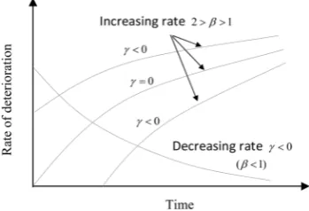
β t> , having exponential and Rayleigh as submodels, is often used for modeling lifetime data. When modeling monotone hazard rates, the Weibull distribution may be an ini-tial choice because of its negatively and positively skewed density shape. Rinne [16] suggested that a three-parameter generalization of the Weibull distribution deals with general situations in modeling survival process with various shapes in the hazard function. Chakrabarty et al. [17] provided rationale for considering three-parameter Weibull deterioration rate. They discovered that many products that start deteriorating appreciably only after a certain period (e.g. after they are produced) and for which the rate of deterioration increases over time have a de-terioration rate best described by a Weibull distribution (Figure 2).1.6. Negative Exponential Distribution
The low flow of traffic can be modeled using the negative exponential distribu-tion. The probability density of the negative exponential distribution is given as
( )
e t, 0f t =λ −λ t≥ (3)
where
λ
is a parameter that determines the shape of the distribution. Figure 3displays the exponential distribution for some values of
λ
.We observe that the probability that the random variable t is greater than or equal to zero is given by;
(
0)
0( )
d 0 e td 1p t≥ =
∫
∞f t t=∫
∞λ −λ t=The probability that the random variable t is greater than a specific value h is
(
)
1(
)
1 0h e td e hp t≥h = −p t<h = −
∫
λ −λ t= −λDOI: 10.4236/am.2019.109052 733 Applied Mathematics Figure 2. Rate of deterioration-time relationship
for a three-parameter Weibull distribution.
Figure 3. Graphical profile of the negative expo-nential distribution for various values of λ.
1.7. Notations and Assumptions of the Model
We adopt the following notations and assumptions in the derivation of our model.
Notations:
1
c: inventory holding cost per unit per unit time.
2
c : shortage cost per unit per unit time.
3
c : ordering cost per order.
4
c : unit purchasing cost.
( )
D t : demand rate at any time, t≥0. T: cycle time.
0
I : initial inventory size.
( )
(
)
1t t β
θ αβ γ −
= − : instantaneous rate function for a three-parameter Wei-bull distribution; where
α
is the scale parameter, β is the shape parameter andγ
is the location parameter. Also, 0<α
1.1
t : time during which there is no shortage.
κ: a constant value between 0 and 1. *
T : optimal value of T. *
0
I : optimal value of I0. *
1
t : optimal value of t1.
*
κ : optimal value of κ .
Assumptions
[image:6.595.278.472.236.341.2]DOI: 10.4236/am.2019.109052 734 Applied Mathematics 2) The planning horizon is infinite.
3) The demand rate is stochastic and given by the negative exponential distri-bution as a function of time t, i.e. D t
( )
=λ
e−λt, whereλ
>0, is the parameter of the distribution.4) Shortages in the inventory are allowed and completely backlogged. 5) The supply is instantaneous and the lead time is zero.
6) Deteriorated unit is not repaired or replaced during a given cycle.
7) The holding cost, ordering cost, shortage cost and unit cost remain con-stant over time.
8) There are no quantity discounts.
9) The distribution of the time to deterioration of the items follows the three-parameter Weibull distribution, i.e.
( )
(
)
1(
(
)
)
exp , 0
W t =
αβ
t−γ
β− −α
t−γ
β t> . The instantaneous rate function is( )
(
)
1t t β
θ αβ γ −
= − .
2. Mathematical Formulation of the Model
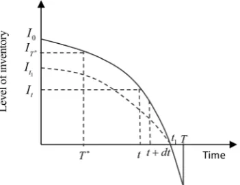
At the beginning of the cycle, the inventory level I t
( )
reaches its maximum( )
0 0I =I units of item at time t=0. During the interval
[ ]
0,t1 , the inventory [image:7.595.288.464.554.689.2]level depletes due to the combine effects of demand and deterioration. At t=t1, the inventory level is zero and all the demand hereafter (i.e. T−t1) is completely backlogged. The total number of backordered items is replaced by the next rep-lenishment. A graphical representation of this inventory system is depicted in Figure 4. Since the depletion of the units is due to demand and deterioration, the rate of change of the inventory level at any time t is governed by the differen-tial equations:
( )
( ) ( )
( )
( )
1 d
, 0 d
I t
t I t P t D t t t
t +
θ
= − ≤ < (4)with boundary conditions I
( )
0 =I0 and I t( )
1 =0. Furthermore the produc-tion rate P t( )
is zero in this case, thus in the interval 0≤ <t t1, the initial value problem to be solved is;DOI: 10.4236/am.2019.109052 735 Applied Mathematics
( )
( ) ( )
( )
( )
( )
0 1
d
, 0 , 0 d
I t
t I t D t I I I t
t +
θ
= − = = (5)In the interval t1≤ ≤t T, the initial value problem becomes;
( )
( ) ( )
1 d
, 0 d
I t
D t I t
t = − = (6)
Employing the previously stated assumptions, we have:
( )
(
)
1( )
1 d
e , 0 d
t I t
t I t t t
t
β λ
αβ
γ
−λ
−+ − = − ≤ < (7)
( )
1 d e , d t I tt t T
t
λ
λ
−= − ≤ ≤ (8)
2.1. Solution of the Model
Equation (7) is a first order differential equation and its integrating factor is:
(
)
1 ( )expαβ
∫
t−γ β− dt=eαt−γβ (9)( )
( ) ( )d
e e e
d
t t t
I t t
β β
α −γ λ −λ α −γ
= −
( )
( ) 1 ( )1
e e d
t t
t t t
t t
I t t
β β
α −γ λ − +λ α −γ
∴ = −
∫
Taking first order approximation of the integrand, we have
( )
{
(
)
}
(
)
e− +λ αt t−γβ ≈ + − +1 λ αt t−γ β = −1 λ αt+ t−γ β
( )
( )( )
( )(
)
{
}
(
)
(
)
(
)(
)
(
)
(
)
1 1 11 1 2 2 2
1 1 1 1
e e
1 d
2 2 2
2 1
t t
t t
I t I t
t t t
t t t t t t t t
β β
α γ α γ
β
β β
λ λ α γ
αλ γ γ λ β λ λ βλ
β − − + + ⇒ − = − − + − − − − + − − − + − − = +
∫
Applying the boundary condition I t
( )
1 =0, we get( )
( )(
)
(
)
(
)(
)
(
)
(
)
1 1 2 2 2
1 1 1 1
e
2 2 2
2 1
t I t
t t t t t t t t
β α γ
β β
αλ
γ
γ
λ
β λ λ
βλ
β
− + + − − − + − − − + − − = +( )
(
)
(
)
(
(
)(
)
)
(
)
( )1 1 2 2 2
1 1 1 1
2 2 2
e
2 1
t
t t t t t t t t
I t β
β β
α γ
αλ γ γ λ β λ λ βλ
β + + − − − − − + − − − + − − ⇒ = + (10) Hence
( )
( )
(
)
(
)
(
)
( )1 1 2 2
1 1 1 1
0
2 2 2
0 e
2 1
t t t t
I I β
β β
α γ
αλ γ γ λ β λ βλ
β + + − − − − − − − + + = =
+ (11)
DOI: 10.4236/am.2019.109052 736 Applied Mathematics
( )
11 1
1
1
e d e e e
t t
t t t t t
t t
t
I t λ λ t λ λ λ λ
λ − − − − = − = − − = −
∫
( )
e t e t1I t −λ −λ
∴ = − (12)
Hence, the inventory level at any time t∈
[ ]
0,T is given by( )
(
)
(
)
(
(
)(
)
)
(
)
( )1
1 1 2 2 2
1 1 1 1
1
2 2 2
e 0 2 1 e e t t t
t t t t t t t t
t t I t β β β α γ λ λ
αλ γ γ λ β λ λ βλ
β + + − − − − − − − + − − − + − −
≤ <
= +
− t1 t T
≤ ≤ (13)
The total cost per unit time, φ
(
T t,1)
, of the inventory system consist of the deterioration cost (DC), the shortage cost (SC), the holding cost (HC) and the ordering cost (OC). Put differently, the total cost per unit time is:(
1)
(
)
1 ,
T t DC SC HC OC
T
φ = + + + (14)
We derive the components of the total relevant cost as follows:
The total quantity of deteriorated items in the time interval
[ ]
0,t1 is given by[ ]
(
)
1 1
1
0 0 0
Initial inventory Total demand within 0,
e d 1 e
t t t
D t
I λ −λ t I −λ
= −
= −
∫
= − − (15)Thus, the deterioration cost per unit time is
(
1)
1 0 1 e
t
DC=c I − + −λ (16)
The average shortage cost within
[ ]
t T1, is(
)
(
)
11
2
2 e d 1 1 e e
T t t T
t
c
SC c λ λ T t t λT λt λ λ
λ −
− −
=
∫
− = − − + (17)The average inventory holding cost accumulated over the period
[ ]
0,t1 is:( )
1
3 0 d
t
HC=c
∫
I t t (18)The total inventory cost per unit time is:
(
)
(
1)
2(
)
1 1( )
1 1 0 1 3 0 4
1
, 1 e t c 1 e t e T t d
T t c I T t c I t t c
T
λ λ λ
φ λ λ
λ
− − −
= − + + − − + + +
∫
(19)Here c c c1, 2, 3 are constants as well as c4 the ordering cost, assumed con-stant.
We assume t1=κT; 0< <
κ
1. This assumption appears reasonable since the length of the shortage interval is a fraction of the cycle time. Substituting1
t =κT in Equation (19), we get:
(
)
(
)
2(
)
( )
1 0 3 0 4
1
, 1 e T c 1 e T e T T d
T c I T T c I t t c
T
κ
κ λκ λκ λ
φ κ λ λκ
λ
− − −
= − + + − − + + +
∫
(20)( )
(
)
(
)
(
)
( )1 1 2 2 2
0
2 2 2
e
2 1
T T T T
I β
β β
α γ
κ αλ γ κ γ λκ β λκ βλ κ
β + + − − − − − − − + + = + (21)
av-DOI: 10.4236/am.2019.109052 737 Applied Mathematics erage cost per unit time φ
(
T,κ)
is now a function of two variables T and κ,its partial derivatives with respect to T and κ are computed and the result
equated to zero. We have
(
)
(
)
( )
0 2
1
3 0 4
1 e
, 1 e e
d
T
T T
T
I c
T c T T
T T T T T T
c I t t c T
κ λκ
λκ λ
κ
φ κ λ λκ
λ − − − ∂ ∂ = +∂ + ∂ − − + ∂ ∂ ∂ ∂ ∂ ∂ ∂ + + ∂
∫
( )(
)
(
)
2 2 2 2(
)(
)
0 e 2 2 2 2 1
2 1
I
T T T T
T
β
α γ κ
β
κλ β κλ κ λ κ λ β ακλ β κ γ
β
− −
∂
= − + − − + + −
∂ + (22)
(
T T 1 e)
T e T(
1)
e T(
T T 1)
T
λκ λκ λκ
λ λκ − λ − κ λκ − λκ λ
∂ − − = − − − +
∂ (23)
The Lebnitz rule for differentiating the integral
( )
(
)
( ) ( )
, d
b a
I f x x
α
α
α =
∫
α isgiv-en by
( )
(
)
(
)
(
)
d d d ,
, , d
d d d
b a
I b a f x
f b f b x
α α
α α
α α α α
∂
= − +
∂
∫
Applying this rule to 0TI t T
( )
, dt Tκ
∂
∂
∫
, we get( )
( )
(
)
0 , d 0 , d ,
T T
I t T t I t T t I T
T T
κ κ
κ κ
∂ = ∂ +
∂
∫
∫
∂ (24)Hence
(
)
(
( ))
(
)
(
)(
)
(
)
(
)
( )
(
)
2 2 2 2
1
2
3 0
e 1
, 2 2 2
2 1
2 1 e
e 1 e 1 e
, d ,
0
T
T T T
T
c
T T T T
T T
T
c
T T
c I t T t I T T
β
α γ
β λκ
λκ λκ λ
κ
φ κ κλ β κλ κ λ κ λ β
β
ακλ β κ γ λκ
λ κ λκ λκ λ λ
λ κ κ − − − − − − ∂ = − + − − ∂ + + + − − + − − − + − ∂ + ∂ + =
∫
(25) Similarly;(
)
(
)
( )
0 2 1 3 0 1 e, 1 e e
d
T
T T
T
I c
T c T T
T
c I t t
κ λκ
λκ λ
κ
φ κ λ λκ
κ κ κ λ κ κ
κ − − − ∂ ∂ = +∂ + ∂ − − + ∂ ∂ ∂ ∂ ∂ ∂ ∂ + ∂
∫
( )(
)
(
)
2 2 2 2(
)(
)
0 e 2 2 2 2 1
2 1
I
T T T T T T
β
α γ κ
β
λ β κλ κλ κβλ αλ β κ γ
κ β
− −
∂ = − + − − + + −
∂ + (26)
(
λT λκT 1 e)
λκT λTeλκT λ λκT(
T λT 1 e)
λκTκ − − −
∂ − − = − − − +
DOI: 10.4236/am.2019.109052 738 Applied Mathematics and
( )
( )
(
)
0 , d 0 , d ,
T T
I t T t I t T t TI T
κ κ
κ
κ κ
∂ = ∂ +
∂
∫
∫
∂ (29)Hence
(
)
(
( ))
(
)
(
)(
)
(
)
( )
(
)
2 2 2 2
1
2
3 0
e 1
, 2 2 2
2 1
2 1 e
e 1 e
, d ,
0
T
T T
T
c
T T T T T
T
T T
c
T T T T
c I t T t TI T β
α γ
β λκ
λκ λκ
κ
φ κ λ β κλ κλ κβλ
κ β
αλ β κ γ λκ
λ λ λκ λ
λ κ κ − − − − − ∂ = − + − − ∂ + + + − − + − − − + ∂ + + ∂ =
∫
(30) where( )
(
)
(
)
(
(
)(
)
)
(
)
( )1 1 2 2 2 2
2 2 2
, e
2 1
t
t T t T t T t T
I t T β
β β
α γ
αλ γ κ γ λ κ β λ λκ βλ κ
β + + − − − − − + − − − + − − = + and
( )
(
)
(
(
)
)
(
)(
)
( )( )
(
)
(
(
)
)
(
)(
)
( )2 2 2
2 2 2
2 2 2 2 1
, e
2 1
2 2 2 2 1
, e
2 1
t
t
t T t T T T
I t T T
T t T T t T T T T
I t T
β β β α γ β α γ
κλ κ κλ β λ κλ βκ λ ακβ β κ γ
β
λ κ λ β λ κλ βκλ αβ β κ γ
κ β − − − − ∂ − + − − + − + + − = − ∂ + − + − − + − + + − ∂ = − ∂ +
2.2. Remark
Equations (25) and (30) provide the necessary condition for *
T and κ* to be minimum points of φ
(
T,κ)
.The sufficient condition for these values to minimize φ
(
T,κ)
is that theHesssian matrix H must be positive definite. Here
(
)
2 2 2 2 2 2 2, T T
H T T
φ
φ
κ
φ
κ
φ
φ
κ
κ
∂ ∂ ∂ ∂ ∂ = ∇ = ∂ ∂ ∂ ∂ ∂ Thus the sufficient condition for optimality is 22 0, 22 0
T
φ
φ
κ
∂ > ∂ >
∂ ∂ and
2
2 2 2
2 2 0
T T
φ φ φ
κ κ
∂ ∂ − ∂ >
∂ ∂
∂ ∂ .
Since I t
( )
=e−λt −e−λt1 for1
t ≤ ≤t T, the total back-order quantity for the
cycle is * *
1
* *
0 e e
t T
I =I + −λ − −λ .
2.3. Optimal Inventory Policy for the Model
DOI: 10.4236/am.2019.109052 739 Applied Mathematics The procedure for reaching this optimum policy is also given. The optimal in-ventory policy for the proposed model is:
Order *
I units for every *
T time units. Use e−λT*−e−λt1* units to offset
the backordered quantity and begin a new cycle with I0
κ units. The total
in-ventory cost per unit time associated with the proposed model is:
(
)
{
(
)
(
)
( )
1 0
2
3 0 4
1
, 1 e
1 e e
d T
T T
T
T c I
T c
T T
c I t t c
κ λκ
λκ λ
κ
φ κ
λ λκ
λ
−
− −
= − +
+ − − +
+ +
∫
2.4. Solution Algorithm
We give the following steps for computing the optimal ordering quantity, op-timal cycle time and the opop-timal total cost for the model:
Step 1: Solve Equations (25) and (30) simultaneously to get the optimal values *
T and κ* for T and κ respectively. Step 2: If at *
T and κ* the sufficiency condition is satisfied, then go to step 3 else stop and declare the solution infeasible.
Step 3: Substitute *
T and κ* into t1 =κT to obtain * 1
t .
Step 4: Determine the optimal EOQ * 0
I by substituting the values of T* and κ* into Equation (11).
Step 5: Substitute the values of * 0
I , T* and κ* into Equation (20) to get the optimal total average cost φ
(
T,κ)
.2.5. Numerical Analysis and Results
In this section we employ MathCAD 14 [18] to obtain numerical solution to the highly nonlinear system of Equations (25) and (30). This will provide us with the optimal solutions for the average cost function for some specified data. We con-sider the following inventory data adapted from Ghosh and Chaudhuri (2004):
1 2.40
c = , c2=5, c3=100.00 , c4 =20.00,
α
=0.001, β =8, γ =0.1, 0.1λ
= ,κ
=0.85,T
=
2
.The format for the MathCAD 14 solve block follows; • Initial values for the unknown variables
(
κ,T)
.• Given.
• Equation 1. • Equation 2. • Find
(
κ,T)
.2.6. Mathcad Solve Block Solution
1: 2.40 2: 5 3: 100 : 0.01 : 8 : 1.5 : 0.4
c = c = c = α = β = λ = γ =
: 0.85 : 2 Initial values of the variablesT
κ = =
DOI: 10.4236/am.2019.109052 740 Applied Mathematics
( )
(
)
(
)
(
) (
)
(
)
(
) (
)
(
) (
)
(
)
( )
(
)
(
)
1 2 2 2 2
2
3
0
2 exp
2 2 2 2 1
2 1
exp exp 1 exp 1 exp
1
exp
2 1
T c
T T T T
c
T T T T T T
c t t t β β κ β α γ
κ λ β κ λ κ λ κ λ β α λ κ β κ γ
β
λ κ λ κ λ λ κ κ λ κ λ κ λ κ λ λ λ
λ
λ λ α γ
β
κ λ κ
⋅ ⋅ − ⋅ − ⋅ ⋅ ⋅ ⋅ − ⋅ ⋅ + − ⋅ ⋅ − ⋅ ⋅ ⋅ ⋅ + ⋅ ⋅ ⋅ ⋅ + ⋅ ⋅ − ⋅ + − ⋅ ⋅ − ⋅ ⋅ + ⋅ ⋅ − ⋅ ⋅ ⋅ − − ⋅ ⋅ − ⋅ ⋅ ⋅ ⋅ ⋅ − ⋅ + − ⋅ − ⋅ − ⋅ + ⋅ ⋅ − ⋅ − ⋅ − ⋅ + ⋅ ⋅ − ⋅
∫
(
)
(
)
(
) (
)
(
)
(
)
(
)(
)
(
)
(
)
2 21 1 2 2 2 2
2 2 2 2 1 d
2 2 2
0
2 1
T t t T T t
T T T T
β
β β
κ λ β λ κ λ β κ λ α κ β β κ γ
α λ κ γ κ γ λ κ κ β λ κ λ κ β λ κ κ
κ β + + + ⋅ ⋅ − ⋅ + ⋅ ⋅ + − ⋅ ⋅ ⋅ ⋅ + ⋅ ⋅ ⋅ + ⋅ ⋅ − ⋅ ⋅ ⋅ − − ⋅ − + ⋅ − ⋅ ⋅ − ⋅ − ⋅ ⋅ + − ⋅ ⋅ − ⋅ + ⋅ = ⋅ +
( )
(
)
(
)
(
) (
)
(
)
(
)
(
) (
)
( )
(
)
(
)
(
)
12 2 2 2
2
3
0
2 exp
2 2 2 2 1
2 1
exp exp exp 1
1 exp 2 1 2 T c
T T T T T T
c
T T T T T T T
c
t t
T t T T t
β
β
κ
β
α γ
λ β κ λ κ λ κ β λ α λ β κ γ
β
λ κ λ λ λ κ λ λ κ λ κ λ
λ
λ λ α γ
β
λ κ λ β λ
⋅ ⋅ − ⋅ − ⋅ ⋅ ⋅ ⋅ − ⋅ ⋅ + − ⋅ ⋅ − ⋅ ⋅ ⋅ ⋅ + ⋅ ⋅ ⋅ ⋅ + ⋅ − ⋅ + − ⋅ ⋅ − ⋅ + ⋅ − ⋅ ⋅ − ⋅ ⋅ − ⋅ ⋅ − ⋅ ⋅ ⋅ ⋅ ⋅ − ⋅ + − ⋅ + ⋅ ⋅ − ⋅ − ⋅ − ⋅ + ⋅ ⋅ ⋅ − ⋅ + ⋅ ⋅ ⋅ − ⋅
∫
(
)
(
) (
)
(
)
(
)
(
)(
)
(
)
(
)
2 21 1 2 2 2 2
2 2 2 1 d
2 2 2
0
2 1
T T T T t
T T T T
T
β
β β
κ λ β κ λ α β β κ γ
α λ κ γ κ γ λ κ κ β λ κ λ κ β λ κ κ
β + + − ⋅ ⋅ + − ⋅ ⋅ ⋅ ⋅ + ⋅ ⋅ ⋅ ⋅ + ⋅ ⋅ − ⋅ ⋅ ⋅ − − ⋅ − + ⋅ − ⋅ ⋅ − ⋅ − ⋅ ⋅ + − ⋅ ⋅ − ⋅ + ⋅ = ⋅ +
(
)
0.9460303,
2.0306513
T
κ =
Find
2.7. Remark
• From the solve block solution we obtain the optimal *
T and κ* as
*
2.0306513
T = , *
0.9460303
κ = .
• It is not difficult to show, using MathCAD, that for these optimal values the sufficient conditions for minimizing φ
(
T,κ)
are satisfied.• We proceed to use these values to compute the optimal * 1
t and I0* to be
*
1 1.921,
t =κ∗ ∗T =
( )
(
)
(
)
(
)
( )1
1 2 2
1 1 1 1
* 0
2 2 2
e 1.197
2 1
t t t t
I β
β β
α γ
αλ
γ
γ
λ
β λ
βλ
β
+ + ∗ ∗ ∗ ∗ − − − − − − − + + = = +• Finally, we have;
(
)
(
)
(
)
( )
}
2
1 0
3 0 4
1
, 1 e 1 e e
d
11.334
T T T
T
c
T c I T T
T
c I t t c
κ λκ λκ λ
κ
φ κ λ λκ
λ − − − = − + + − − + + + =
∫
DOI: 10.4236/am.2019.109052 741 Applied Mathematics dependent three-parameter Weibull deterioration and a stochastic type demand in the form of a negative exponential distribution, we obtained the following re-sults.
The optimum cycle time *
2.031
T = days.
The optimum value *
0.94603
κ = .
The optimum stock-period *
1 1.921
t = days.
The economic order quantity *
0 1.197
I = units.
The optimum total average cost
(
)
*, $11.334
T
φ κ = per day.
The optimum number of order, N*=1 1.197=0.8354 order per day.
2.8. Conclusions
In this work we developed an inventory model for a three-parameter Weibull deteriorating items with stochastic demand in the form of a negative exponential distribution. We derived the optimal inventory policy for the proposed model and also established the necessary and sufficient conditions for the optimal poli-cy. In the solution of the differential equation obtained, because of the cumber-some nature of the associated integral, we were forced to make a first order approximation for the integrand involving an exponential function. This in turn enabled us to obtain a closed form solution for our model. We provided a numerical example illustrating our solution procedure. Though our solution is only approximate, we were still able to obtain very reasonable results which compared favourably with that of Ghosh and Chaudhuri [6] (T*=2.145 days,
*
0.8832
κ = ) for the deterministic demand case.
It is important to state that the numerical procedure for this problem relied heavily on the power of MathCAD14, which was used to solve a highly nonlinear system of equations in two unknowns, and involving a definite integral. The ad-vantage of this numerical software is that the equations are composed as they appear in the text and need not be recast in a special format for computation.
Conflicts of Interest
The authors declare no conflicts of interest regarding the publication of this pa-per.
References
[1] Ritchie, E. (1980) Practical Inventory Replenishment Policies for a Linear in De-mand Followed by a Period of Steady DeDe-mand. Journal of the Operational Research Society, 31, 605-613.https://doi.org/10.1057/jors.1980.118
[2] Gupta, P.K. and Hira, D.S. (2002) Operations Research. S. Chand & Company Ltd., New Delhi.
[3] Rinne, H. (2009) The Weibull Distribution: A Handbook. Chapman & Hall/CRC, Boca Raton.
DOI: 10.4236/am.2019.109052 742 Applied Mathematics [5] Ghare, P.M. and Schrader, G.H. (1963) A Model for Exponentially Decaying
In-ventory System. Journal of Industrial Engineering, 14, 238-243.
[6] Ghosh, S.K. and Chaudhuri, K.S. (2004) An Order-Level Inventory Model for a De-teriorating Item with Weibull Distribution Deterioration, Time-Quadratic Demand and Shortages. Advanced Modeling and Optimization, 6, 21-35.
[7] Dave, U. (1986) An Order Level Inventory for Items with Variable Instantaneous Demand and Discrete Opportunities for Replenishment. Opsearch, 23, 244-249. [8] Li, R., Lan, H. and Mawhhinney, J.R. (2010) A Review on Deteriorating Inventory
Study. Journal of Service Science and Management, 3, 117-129. https://doi.org/10.4236/jssm.2010.31015
[9] Khanra, S., Ghosh, S.K. and Chaudhuri, K.S. (2011) An EOQ Model for a Deteri-orating Item with Time Dependent Quadratic Demand under Permissible Delay in Payment. Applied Mathematics and Computation, 218, 1-9.
https://doi.org/10.1016/j.amc.2011.04.062
[10] Bakker, M., Riezebos, J. and Teunter, R.H. (2012) Review of Inventory Systems with Deterioration since 2001. EuropeanJournalofOperationalResearch, 221, 275-284. https://doi.org/10.1016/j.ejor.2012.03.004
[11] Goyal, S. and Giri, B.C. (2001) Recent Trends in Modeling of Deteriorating Inven-tory. EuropeanJournalofOperationalResearch, 134, 1-16.
https://doi.org/10.1016/S0377-2217(00)00248-4
[12] Ravichandran, N. and Srinivasan, S.K. (1988) Multi-Item (S,S) Inventory Model with Poisson Demand, General Lead Time and Adjustable Reorder Time. IIMA Working Papers WP 1988-08-01_00838, Indian Institute of Management Ahmeda-bad, Research and Publication Department.
[13] Weiss, H.J. (1995) Stochastic Analysis of a Continuous Review Perishable Inventory System with Positive Lead Time and Poisson Demand. European Journal of Opera-tions Research, 84, 444-457.https://doi.org/10.1016/0377-2217(93)E0254-U
[14] Aggoun, L., Benkerouf, L. and Boumenir, A. (2001) A Stochastic Inventory Model with Stock Dependent Items. Journal of Applied Mathematica and Stochastic Anal-ysis, 14, 317-328.https://doi.org/10.1155/S1048953301000284
[15] Lian, Z., Zhao, N. and Liu, X. (2009) A Perishable Inventory Model with Markovian Renewal Demands. International Journal of Production Economics, 121, 176-182. https://doi.org/10.1016/j.ijpe.2009.04.026
[16] Rinne, H. (2009) The Weibull Distribution: A Handbook. Chapman & Hall/CRC, Boca Raton.https://doi.org/10.1201/9781420087444
[17] Chakrabarty, T., Giri, B.C. and Chaudhuri, K.S. (1998) An EOQ Model for Items with Weibull Distribution Deterioration, Shortages and Trended Demand: An Ex-tension of Philip’s Model. Computers & Operations Research, 25, 649-657. https://doi.org/10.1016/S0305-0548(97)00081-6