A Solution to the Famous “Twin’s Problem”

(1)

ISSN Online: 2160-0384 ISSN Print: 2160-0368

DOI: 10.4236/apm.2019.99038 Sep. 24, 2019 794 Advances in Pure Mathematics

A Solution to the Famous “Twin’s Problem”

Prodromos Char. Papadopoulos

The 1st Gymnasium in Yiannitsa City, Yiannitsa, Greece

Abstract

In the following pages I will try to give a solution to this very known unsolved problem of theory of numbers. The solution is given here with an important analysis of the proof of formula (4.18), with the introduction of special inter-vals between square of prime numbers that I call silver interinter-vals δM. And I

make introduction of another also new mathematic phenomenon of logical proposition “In mathematics nothing happens without reason” for which I use the ancient Greek term “catholic information”. From the theorem of prime numbers we know that the expected multitude of prime numbers in an interval

[

x x dx, +

]

_{is given by formula}π

( )

x _dx ln

( )

x _{considering that}

interval as a continuous distribution of real numbers that represents an ele-mentary natural numbers interval. From that we find that in the eleele-mentary interval

[

ν ν, +1

)

around of a natural number ν we easily get by dx=1 the probability p

( )

ν 1 ln

( )

ν that has the ν to be a prime number. From the last formula one can see that the second part p

( )

ν >1 8

( )

ν of formula (4.18) is absolutely in agreement with the above theorem of prime numbers. But the benefit of the (4.18) is that this formula enables correct calculations in set N on finding the multitude of twin prime numbers, in contrary of the above logarithmic relation which is an approximation and must tend to be correct as ν tends to infinity. Using the relationship (4.18) we calculate here the multitude of twins in N, concluding that this multitude tends to infinite. But for the validity of the computation, the distribution of the primes in a random silver interval δM is examined, proving on the basis of catholic

in-formation that the density of primes in the same random silver interval δM

is statistically constant. Below, in introduction, we will define this concept of “catholic information” stems of “information theory” [1] and it is defined to use only general forms in set N, because these represent the set N and not fi-nite parts of it. This concept must be correlated to Riemann Hypothesis.

Keywords

Twin Problem, Twin’s Problem, Unsolved Mathematical Problems, Prime

How to cite this paper: Papadopoulos, P. (2019) A Solution to the Famous “Twin’s Problem”. Advances in Pure Mathematics, 9, 794-826.

https://doi.org/10.4236/apm.2019.99038

Received: August 13, 2019 Accepted: September 21, 2019 Published: September 24, 2019

http://creativecommons.org/licenses/by/4.0/

(2)

DOI: 10.4236/apm.2019.99038 795 Advances in Pure Mathematics Number Problems, Millennium Problems, Riemann Hypothesis, Riemann’s Hypothesis, Number Theory, Information Theory, Probabilities, Statistics

Stay away from infinity Never look it in the eye

Friedrich Gauss

1. Introduction

The symbol qν (with

ν ∈

N

) from now on will symbolize the prime numbers.

There are the definitions of the endless sequence of the prime numbers that will be symbolized as follows: q0=1,q1=2,q2=3,q3=5,.

Let a random natural number aν =ν,

ν ∈

N

and let two more prime

num-bers qα, qβ that are not equal to each other, qα ≠qβ. At first, it will be shown

the independency of the fact that “the random Natural number aν, can be

di-vided by the prime number qα” from the fact that “the random Natural number

aν can be divided by the prime number qβ”. Let, also, without impairment of

the generality of this proof, that qα =7 and qβ =5. Obviously, per 35

succes-sive Natural numbers the 5 Natural numbers will be multiple of 7 and the 7 Natu-ral numbers will be multiples of 5 and only one NatuNatu-ral number will be multiple of both 7 and 5. So, when selecting an Integer number aν from the infinite

multi-tude of Natural numbers, the information of the fact that “aν is multiple of 7”

does not interfere with the probability of the fact that “aν is multiple of 5”

be-cause every five multiples of 7 there will be only one that can be divided once again by the prime number 5, regardless of the information of the first fact. The Natural number aν will indeed belong to a group of thirty-five, if the

multi-tude of Natural number N is divided into groups of thirty-five successive Natural numbers. Therefore, if the first fact, “aν is multiple of 7”, is valid then aν will

belong to the group of 5 (of a group of 35) that are multiples of 7. This group of 5, however will include only one multiple of 5, therefore aν will again have 1/5

probability of being multiple of 5, regardless of the information of the first fact that “it is multiple of 7”. The proof is obviously generalized with the same me-thodology for any of the prime number qα, qβ, not equal to each other.

It should be underlined that the Natural number 0 is divided by every Natural number, even when selecting a random integer aν, which will obviously have a

probability equal to 1qk of being divided by the prime number qk. Here, the

probability has the meaning of the appearance frequency of a subset of Natural numbers, so when stating that fact Γ is independent of the probability-frequency that is referring to the subset of these Natural numbers, defined; based on an ac-tivity-criterion of their selection, it is meant that fact Γ is independent from the activity-criterion of their selection.

Opposite to that now, the information “a Natural number aν is divided by

(3)

DOI: 10.4236/apm.2019.99038 796 Advances in Pure Mathematics and 3, since _{18 2 3}_{= ⋅}1 2_{, (or generally}_{18 2 3 5 7 11 13}1 2 0 0 0 0 0

k

q

= ⋅ ⋅ ⋅ ⋅ ⋅ _{ }_{). The}

sentence that was just shown is directly understood by writing the general form of a random Natural number aν = v:

3 1 2 1 2 3

k k

j j j j

i i i i

aν =q q q q

where j j1, , ,2 jk are Natural, non-zero numbers.

Therefore, the fact “aν is divided by the prime number q nn, ∈

{

i i i1 2 3, , , , ik

}

” will be independent from the fact “the Natural number aν is divided by the

prime number q mm, ∈

{

i i i1 2 3, , , , ik

}

” if m n≠ . This will be name Proposition of Divisibility Independence (PDI), which as shown is valid for the set N of Nat-ural numbers.

Every random element selection from a given set A will be called Catholic Se-lection (CS), a term from ancient Greek language. In addition, as Catholic in-formation will be defined a set K of catholic (logical) propositions that will be valid for infinity CS elements from different appropriate subsets (of finite mul-titude) of a set A. For example, a set K consisting of finite multitude of relations (written in general form) among infinite elements of another set A. An example of a logical proposition (or simply a proposition) that is a Catholic Proposition (CP), due to the fact that it is valid for infinite elements in N, specifically for in-finite pairs of multiples of two prime numbers each time, is the PDI. The set of all the CP, meaning the propositions of catholic cardinality in N, that can be proved using PDI will now defined as catholic information of PDI for N. Owing that in mathematics nothing happens without a reason, it is concluded that if an algorithm of creation of a set A with infinite multitude is proven that does not create a property (proposition) P that will be catholically valid in A, therefore not implied by this algorithm (a set of finite multitude propositions) that the proposition P (e.g. a non-random statistical distribution) is valid in A, then P will not be valid in A. This last sentence will be named Proposition of Catholic Information.

1.1. The Fundamental Principles of This Research

They are: 1) The introduction of “catholic information” that we introduced above. 2) The extraction of all possible catholic or general relationships for which we define to must being them valid in all parts of set of natural numbers N and not only for special parts [2]. So the catholic formulas must use alphanu-merical (by general expression) symbols for their catholic variables. 3) The defi-nition of two kinds of intervals which we here call silvers and darks respectively. 4) The statistical calculation of catholic multitude of twin prime numbers in set N that is a calculation until infinity.

1.2. About the Study

(4)

DOI: 10.4236/apm.2019.99038 797 Advances in Pure Mathematics concept and by use of (2.1), (4.18) we solve the problem in two ways: First by compact calculation using the appearance frequencies of twins in N, and second by using the dark intervals of N, which are increasing their sizes by a monster rate and however they are have infinite multitude. In this last process we initially proof that if some intervals not includes twin primes then this hypothesis drives to the existence of one twin prime on every top of these intervals. Thus we again arrive on the same conclusion. In pages before the relation (4.20), we examine the stability of frequency of prime numbers appearance in a random “silver in-terval”, which is, a condition useful of validity of statistical calculations bellow.

1.3. Conclusions

Our conclusions from the below are: 1) The hypothesis of twin prime numbers is correct. 2) Maybe the concept of “catholic information” can be used as well in other Mathematical investigations. This concept is the other expression of fun-damental proposition that “In mathematics nothing happens without reason”. This concept of “catholic information” maybe could be connected by Riemann hypothesis [3] [4].

1.4. Twin Pairs

Here will be studied the twin pair problem. Let that an “honest” dice (in the shape of a normal hexagon) is thrown three consecutive times and the three consecutive positions are noted respectively A/B/Γ. Which twin pairs (meaning repetitions) of a particular number, i.e. of 5, are expected?

Answer [5]:

According to the sample space 6(6)6 = 216 facts there will be five cases of the form 5/5/C, where Γ is one of the results {1, 2, 3, 4, 6}, which has multitude of five. Similarly, there are five cases of the form Α/5/5, where Α is one of the re-sults {1, 2, 3, 4, 6}, and only one is the 5/5/5. Due to the 10 first having 1 twin pair of 5, meaning one boundary “/” for the 5, and the last (one) case having 2 twin pairs, there will be altogether 10(1) + 1(2) = 12 total twin pairs in the 216 cases, and therefore the probability of twin pairs in A, B, Γ facts, (which is “the 5” in each one of the ordered throw) will be 12/216 = 1/18. On the other aspect of the counting method based on the probability p=1 6_{to get number 5 in a} throw, there will be probability _p2 ₌

( )( )

_{1 6 1 6} ₌_{1 36}

(5)

DOI: 10.4236/apm.2019.99038 798 Advances in Pure Mathematics boundaries “/” of the facts of the throws A A1/ 2/ / AN would be:

(

₁

)

2

(

_{1 36}

)

P= N− p = N− (1.1)

One could try to prove this last relation in the case of a/b/c/d using the first method with the sample space. However, in this case the counting of the proba-bility P0 will be completely different in order for at least one of the above facts X and Y to occur. This probability will be counted as follows:

(

)

( )

( ) (

)

0 0 0 0 0 | _{36 36 36 6 216}1 1 1 1 11

P X Y∪ =P X +P Y −P X P Y X = + − =

The probability P Y X0

(

|

)

above is 1/6, because when fact X occurred the information that the second pair has already given 5 is provided, so the

(

)

0 |

P Y X will correspond only to the probability “the third dice will be again 5”, and it is obviously 1/6. In the sample space of the 216 facts there will indeed be 5 + 5 + 1 = 11 of these cases (and not 12 as before), since 5 cases will be of the form 5/5/Γ, the other 5 of the form A/5/5 and only 1 will be 5/5/5. The reader perceives that the differentiator is the key phrase in the above sentence: at least one.

Coming to an end, by proving the independency of the events; the “divisibility of the random natural number aν_{by the random prime number}qα (of its

sub-sequence)” from the “divisibility of the random natural number aµ by the

random prime number qβ (of its sub-sequence)” the definition of these two

events independency will be repeated: Any two events Γ1 and Γ2 will be consi-dered independent from each other in a set (their range) A, “if and only if the frequency-probability of the elements in A where Γ1 appears, is the same as the frequency-probability of the elements in A where Γ1 and Γ2 appear together (once each)” and additionally the last sentence (“…”) is valid if C1 and Γ2 are in-terchanged in it.

2. Specification of the Indefinite Frequency-Probability

Appearance of Prime Numbers

A set YM =

{

q q q1, , , ,2 3 qM

}

is taken as a sub-sequence of the interval

)

2 2 1

, M q qM M

δ _{= } ₊ _{. The internal dm will be named Silver interval. It should also be} clarified the reason why for the study of the natural numbers. The interval δM

will be named Silver Interval.

It should also be clarified the reason why in the study of natural number

M

aν = ∈ν δ the prime numbers qλ were chosen as elements of YM the

nat-ural numbers with the characteristic: It is noticed that if the random natnat-ural number aν is divided by another positive natural number κ > aν , then the

quotient of this division, let natural number μ, will satisfy the relation µ< aν .

It is obvious since µ κ⋅ =aν. In other words, if µ> aν was true, then it

would be aν = ⋅ >µ κ a aν ν =aν, which is absurd. Therefore, if aν has a

di-visor greater than aν then it will also have a divisor smaller than aν ,

which is followed by the fact that is a natural number aν is not divided by

(6)

DOI: 10.4236/apm.2019.99038 799 Advances in Pure Mathematics other prime number greater than aν . Because if this last statement were to be

true, then according to the aforementioned facts there would be a divisor smaller than aν , which would either be prime or it would be analyzed in product of

prime numbers that are for sure smaller than aν . The conclusion drawn is

that in the case where aν, does not have as a divisor a prime number smaller

than aν , then aν is the prime number. Therefore, the prime numbers that

define as possible divisors of aν being prime, are only the prime numbers that

are all smaller than its square root, which is the sub-sequence of prime numbers of aν, that was defined above.

The probability Pν, that aν =ν is not divided by any of the elements of the

sub-sequence of 2,3,5,7, , qMν (defining q0=1,q1=2,q2=3,q3=5,) will

be equal to the products of the probabilities not to be divided by 2,3,5,7, , qMν.

These probabilities will respectively be 1 1,1 1,1 1,1 1, ,1 1 2 3 5 7 qMν

− − − − _ − _{, due to}

the fact that Mν multitude events A A A1, , , ,2 3  AMν that state respectively that

the natural number aν =ν is divided by the prime numbers 2,3,5,7, , qMν

of its sub-sequence, which according to PDI that was previously proven, per two events that are independent from each other. It is obvious that 1/2 is the proba-bility of the natural number aν, to be divided by 2, that is to be an even number

with complimentary probability the 1 − (1/2) not to be divided by 2. Similarly, 1/3 is the probability of aν to be divided by 3, while 1 − (1/3) is the

compli-mentary probability to not be divided by 3 and so on for every term of the sub-sequence. The A A A1, , , ,2 3  AMν, however are not every two exclusive

events from each other, owning to the fact that the divisibility of the natural number aν =ν by a number of its sub-sequence do not exclude its ability to be

divided by another term of that sub-sequence. For example, the natural number

30 30

a = _{has as a sub-sequence of prime numbers 2, 3, 5 and the fact that it can}

be divided by another of these three terms. It is indeed divided by the term 3. The probability Pν of the following Equation (2.1) is a unique enumerate of

prime numbers, but (initially) in not-well-defined intervals. The following defi-nition is derived from the available information of the production of infinite element of set N, provided that according to the definition of Shannon the probability Pν is another way of expressing information. Based on the fact that

the events A A A1, , , ,2 3  AMν are every two independent from each other, one

concludes that the probability-frequency of appearance of all the events above will simply be the product of all their individual probabilities therefore one will obtain the relation.

1 1 1 1 1

2 3 5 7 M

P

q

ν

 

    

= −_ _ − _ − _ − _ _ − _

    _{ }  (2.1)

It will, however be proven and in another way the relation (1.2) [5]. Let Pν

the probability that the natural number aν is divided with at least one term of

(7)

DOI: 10.4236/apm.2019.99038 800 Advances in Pure Mathematics

1

Pν = −Pν′ (2.2)

The probability Pν, for the events A A A1, , , ,2 3  AMν, that are per two

inde-pendent to each other, which state that the given natural number aν is divided,

respectively, by the prime natural numbers 2,3,5,7, , qMν of its sub-sequence,

is:

(

)

( )

(

)

(

)

( )

(

)

1 2 1 2 3

1 2 3

1

1 2 3

1 .

M

j j j j j j

M

P P A A A A

P A P A A P A A A

A A A A _ν

ν ν ν

ν − ′= ′ ∪ ∪ ∪ ∪ ′ ′ ′ = − ∩ + ∩ ∩ − + − ∩ ∩ ∩ ∩

∑

  

and because the facts A A A1, , , ,2 3  AMν are as previously mentioned per two

independent from each other, the relation above becomes

(

j1 j2

)

( ) (

j1 j2| j1

)

( ) ( )

j1 j2

P Aν′ ∩A =P Aν′ ⋅P Aν′ A =P Aν′ ⋅P Aν′

The second part of the equation in the last relation is due to the independency of the fact A Aj₁, j₂. Similarly there is:

(

)

( ) (

)

(

)

( ) ( )

( )

1 2 3 1 2 1 3 2 1

1 2 3

| |

j j j j j j j j j

j j j

P A A A P A P A A P A A A

P A P A P A

ν ν ν ν

ν ν ν

′ ∩ ∩ = ′ ⋅ ′ ′ ∩

′ ′ ′

= ⋅ etc.

So, the probability Pν results to expression

( )

1 2 1 2 3

1

1 2

1 1 1 1 1 1 ₁ M 1 1 1

j j j j j j M

P

q q q q q q q q q _ν

ν ν

−

′ =

∑

−

∑

+

∑

− + −_ ⋅

∑

_ _(2.3)

In the above sums the indicators j j j1, , ,2 3  are as known, per two different

from each other and obviously P Aν′

( )

_j_κ =1q_j_k is the probability, of the event

k

j

A , where the natural number aν is divided by a prime number qjκ =qλ of its sub-sequence.

Let now be the Polynomial

( )

1 2 1 0

1 2 1

M M M

M M

f x x ν a x ν a x ν a x a x

ν ν

− −

−

= + + + + + (2.4)

with roots x x x x x1, , , , , ,2 3 4 5  xMν respectively the fractions

1 1 1 1 1_{, , , , , ,} 1 2 3 5 7 11 qMν



Therefore one has

( )

1 1

(

1 2 3 M

)

f = + a a+ +a ++a ν (2.5)

and now the known polynomials give

1 j 1

j

a x

q

= −

∑

= −

∑

, 1 2

1 2

2 j j 1 1

j j

a x x

q q

= +

∑

=

∑

_(2.6)

and also

( ) (

1

)(

2

) (

M

)

1₂ 1₃ 1

M

f x x x x x x x x x x

q ν ν      = − − − =_ − _ −   −    

  (2.7)

(8)

DOI: 10.4236/apm.2019.99038 801 Advances in Pure Mathematics (2.2) and (2.7) where x = 1 one concludes in (2.1).

The relation above (2.1) indefinitely gives the probability to be equal to the positive natural number aν, because it cannot be in a defined set δ =

[

ν ν1, 2

)

where the probability Pν is counting the exact multitude Qδ of the prime

numbers in it: 2

1

Qδ ν Pν ν

=

∑

_{. The exact counting as shown below, will be done in}

appropriate intervals, that have already been named silver intervals δM, and

with the use of an unknown probability Pν, that will be proven to be greater

than a useful expression, that will be related to (2.1). From the above it is be-coming clear that all the natural number that have the same sub-sequence of prime numbers should constitute an interval such as δM, i.e. the intervals:

(

2 2

)

2 2

)

2 2

)

2 2

)

0 1 ,2 , 1 2 ,3 , 2 3 ,5 , 3 5 ,7

δ = δ =_ δ =_ δ =_

respectively correspond in the sub-sequences of the prime number {(1)}, {(1), 2}, {(1), 2, 3}, and these are defined as the four prime silver intervals that clearly in-clude only the natural numbers. For example the interval δ1 includes a

multi-tude of five numbers. Number one (1) was in purpose set in bracket above so as to declare that number one is not included in the elements of these subsets, be-cause number 1 is not a prime number. It should be clarified that a definition of prime numbers is that prime numbers are all the multiples of number one (therefore they are natural numbers) that have the attribute to not be divided by one another. So the prime numbers define the set of all the possible independent repetitions of number one, since none of them is the repetition of the other. It is noticed that the first of the above silver intervals, that is δ0, has as a

sub-sequence the empty set and includes two prime numbers which are 2 and 3, the second δ1 has as its sub-sequence the unit-set with 2 as an element and

in-cludes two prime numbers, 5 and 7, while the third one inin-cludes five prime numbers, the fourth includes sixteen prime numbers and so on. Furthermore, the enumerators-probabilities that were mentioned, Pν and Pν , will have

constant value in every specific silver interval, which will be explained in details, and be proven in Section 4. In this section it will be defined that these values will be dependent, according to relation (2.1), only on the sub-sequence of prime number, which is the same for all natural numbers and only of the specific silver interval:

constant, constant,

Pν = Pν = ∀ ∈ν δκ,

with κ function of ν.

Now certainly the definition of silver intervals is justified

)

2 2 1

, M M

q q

κ

δ _{= } ₊

And seeing that M M= ν =κ,

∀ ∈

ν

N

one obtains

)

2 2 1

, M q qM M

δ _{= } ₊ _(2.8)

(9)

DOI: 10.4236/apm.2019.99038 802 Advances in Pure Mathematics A check of Pν by calculating the counting of

2

1

Qδ ν Pν

ν ν=

=

∑

_{and with the use}

of a computers, via (2.1) with ν =1 4 and ν2 an arbitrarily large natural

number, it is shown that the countable multitude of prime numbers, whilst at the beginning coincides with the real, it becomes more and more larger than that of the real multitude of prime numbers, as ν2 is increased. The reason why this

is happening will be explained below and will be proven that the new precise probabilityp

( )

ν =Pν, that was mentioned before will tally the precise multitude

of prime numbers: 2

1

Qδ ν Pν

ν ν=

=

∑

, although unknown here, it will satisfy in every

particular silver interval 2 2

)

1

, M q qM M

δ _{= } ₊ _{a very useful inequality, which will be} named fundamental inequality of the silver intervals.

It will also be proven true that for the probability of the relation (2.1): limPν 0

ν →∞ = (2.9)

In the beautiful book “the secret life of numbers” professor of Mathematics Andrew Hodges mentions that one of the smartest tricks in the history of ma-thematics is the Euler transformation below:

1 2 3 1 2 3 1 2 3

1 2 3 4

1 1 1 1 1 1 1 1 1

1 1 1

2 2 2 3 3 3 5 5 5

1 1 1 1 1 1 1 1 1

1 1

2 3 4 5 6

qν qν qν qν

 ₊ ₊ ₊ ₊  ₊ ₊ ₊ ₊  ₊ ₊ ₊ ₊ 

   

   

 

+ + + + + = + + + + + +

 

 

  

   

(2.10)

The second part of 2.10 is the known harmonic sequence that as known is in-exhaustible and corresponds to Riemann’s function:

( )

_z 1 1 1 2 1 3z z z

ζ = + + +_

The proof of (2.10) results directly from the general form of writing the natu-ral number:

3 1 2 1 2 3

k k

j j j j

i i i i

aν =q q q q (2.11)

That was mentioned in the beginning of Section 2. Executing retrospectively the multiplication of the 1st_{part it will indeed lead to the 2}nd_{part due to the} ap-pearance of all the combinations of (2.11) in the denominators, and so all the integers positive numbers etc.

The relation (2.10) is known from the time of Gauss, that leads directly to the conclusion found by Euclid thousands years ago, which is that the prime num-bers are infinite. If they were not then the first part of (2.10) would be a product of finite multitude of derivatives, where each one of them would converge and therefore this product would not deviate from infinity. This however, is absurd, since the second part would also not deviate, which is indeed deviating, because it is the harmonic sequence that was previously mentioned. However, the au-thor’s shorter proof can be given here: “the relation (2.11) includes exponents that are natural integer numbers and therefore each one of them is developed again in the same way 1 2 3

1 2 3 r r

m

m m m

s s s s

(10)

DOI: 10.4236/apm.2019.99038 803 Advances in Pure Mathematics will be developed again in the same way and so on. It is therefore obvious, that if the prime numbers had finite multitude in N, then the combinations for the re-presentation the natural numbers aν would be depleted, since these

combina-tions would not obviously have the advantage of infinite different per-two ma-thematical (tree-like) representations. Hence, in that case the infinite natural numbers would not be represented by the relation (2.11) which is absurd”.

One more not so well known relation of the bibliography (that is also men-tioned in Section 6 of Andrew’s Hodges book) for a random prime number qν,

as symbolized here, is:

1

1 2 3 4

1 1 1 1 1

1 1

qν qν qν qν qν

−

 

− = + + + + +

 

   (2.12)

It is noted that (2.12) could be proven easily from the known Taylor formula-tion [3]:

( )

( ) (

0

) ( ) (

1 0

)

2

( ) (

0

)

3

( )

0 _1! 0 _2! 0 _3! 0

x x x x x x

f x = f x + − f x′ + − f x′′ + − f x′′′ +_

Plugging x0 =0 and

( ) (

)

1

f x = −x − _{, and placing afterwards the}

differen-tiations of x, where x is 1qν . So the same relation which can be used to convert

the functions such as cos

( )

_x ,ex_{etc. was used in a sequence of infinite terms.} Now, because the second part of (2.10) tends towards infinity when

ν

→ ∞_,

as stated before, combining the relations (2.1), (2.10), (2.12) one immediately concludes to the proven (2.9)

The 1st_{part of (2.10) is equal to the function zeta}

( )

1 1 1 1 1 1 1 1 1 1 2 3 4 5 6 7 8

ζ = + + + + + + + + (2.13)

Because when executing the 1st_{part the multiplication in the denominators of} the fractions, all the combinations of the products of all the prime derivatives, raised in all the powers, to infinity will appear. Hence, according to the relation

3 1 2 1 2 3

k k

j j j j

i i i i

aν =q q q q (which was reported in the beginning of this Section 2) the

result will be all the natural numbers, therefore function ζ

( )

1 . Combining this fact with the one from (2.10) (2.12) and also with (2.1) the following known re-lation is concluded:

( )

1 lim 1

P

ν _ν

ζ

→∞

= _(2.14)

3. The Tracker of Infinity (Eratosthenes Sieve)

One should think about the endless axis of positive natural numbers aν, that

(11)

natu-DOI: 10.4236/apm.2019.99038 804 Advances in Pure Mathematics ral number aν send on your right, to the abyssal infinity, a message to the light

blue observers-natural numbers, which are integer multiples of aν, that says

change your colour to black. The aν remains light blue and is registered in

your log book”. What will happen? Simply. In the route

2 3

→

all the even natural numbers will be black to infinity except of course for number 2. These will be called second-multiple (2-multiples) not including number 2. In the route

3 4

→

_{there will be black numbers except from the second-multiples and}

all the multiples of 3 to infinity except for the natural number 3. These multiples of 3 not including the initial number 3 will be called third-multiples (3-multiples) numbers. When the tracker reaches number 4, however, finds it black and does not send a message for colour changing to the observers-natural numbers. Number 5 is found light blue (unmarked) and a new message is sent, according to the order given, to mark all the integer multiples of the natural number 5 ex-cept for 5, with the colour black. The multiples of 5 exex-cept for 5, will be called fifth-multiples numbers and so on. Therefore, the tracker in this journey leaves behind as light blue only the prime numbers that have been registered in the log book. The integers, third-multiples, fifth-multiples, seventh-multiples etc. meaning all the natural numbers that are not prime numbers and have been marked black will be called prime-multiples numbers. According to what was shown regarding the silver interval during the route ₂2_→₃2_{, that is, in the tracker’s route inside}

the silver interval 2 2

)

1 2 ,3

δ _{= } _{, an encounter with all the now blackened} mul-tiples of 2 will take place. The numbers 5, 7 will remain light blue during this route and they are prime numbers. Similarly, during the new route in

)

2 2 2 3 ,5

δ _{= } _{, the tracker will encounter, marked in black, all the multiples of 2} and 3. That means that the multiples of the subsequence of the prime numbers in the silver interval that the tracker crosses each time, will be marked black.

The prime numbers that are integer multiples of the random prime number

s

q , will be called qs-multiples. Additionally, in a random silver interval

)

2 2 1

, M q qM M

δ _{= } ₊ _{the natural numbers will be called:}

2 2 2 2 2

1

, 1, 2, 3, , 1

M M M M M

q q + q + q +  q + −

respectively as 1st_{, 2}nd_{, 3}rd_{, … position in the interval} 2 2

)

1

, M q qM M

δ _{= } ₊ _.

According to this last definition the question now is; which is the position of a first appearing qs-multiple in δM = q qM2, M2+1

)

and which is the position of the last qs-level in this silver interval. This positions are called θs

(

1,M

)

and

(

,

)

s M

θ τ respectively, ensuring that the symbols represent the information given accordingly. Here 1 represents the 1st_and_τ_{represents the last (from the} Greek word “τελευταίος” that means last). The interval

( )

(

1,

) (

, ,

)

s s s

b M = _θ M θ τ M _ that includes only natural numbers will be called band of qs-multiples (prime-multiples) of the silver interval δM. Furthermore,

2 2

1

M M M

d =q + −q symbolizes the “length” of a random silver interval

)

2 2 1

, M q qM M

(12)

(

) ( )

2 2

(

)

2 2

1 2 4 1 4

M M M M M M M

d =q + −q ≥ q + − q = +q > q (3.1)

And since qM ≥qs,∀ =s 1,2,3,4, , M one concludes that:

2 2

1 4 4 , 1,2,3,4, , , 1

M M M M s

d =q + −q > q ≥ q ∀ =s  M ∀M > (3.2)

Also, due to the distance of the origin θ_s

(

1,M

)

of any band b Ms

( )

from

the origin of the silver interval 2 2

)

1

, M q qM M

δ _{= } ₊ _{being always less that the} dis-tance qs of the two successive qs-levels of its subsequence (that means qs≤qM)

there will be:

(

)

(

)

0≤θs 1,M − <1 q ds, M −θ τs ,M <qs, ∀ ≤qs qM (3.3)

The “equal to 0” in the first relation (3.3) represents the case where qs =qM.

For example:

(

1,

)

1, 1

(

1,

)

2, 1

(

,

)

, 1

M M M M dM M

θ = θ = θ τ = ∀ >

Because 2 2 1

, M M

q q + are odd natural numbers as squares of prime numbers (that

are odd). Also, it should be reminded that M M= ν =1,2,3,4,5,6,. Moreover, it will be symbolized as

( )

(

,

)

(

1,

)

1

s s s

l M =θ τ M −θ M +

the “length” of a random band b Ms

( )

. Therefore as an example one finds:

( )

1 M 2 1 M 1, 1

l M =d − + =d − ∀M > , for example l1

( )

2 =16 1 15− =

But l2

( )

2 =16, l3

( )

2 =11, l2

( )

3 =22, l3

( )

3 =21, .

As “lengths” for both the silver intervals and the bands were defined not the geometrical distances of the two ends but the multitude of the natural numbers that are included in the interval that corresponds each time to the silver interval (or band). In contrast, their normal length l Ms

( )

−1 could be named

geome-trical length.

4. The Silver Intervals, the Fundamental Inequality and a

First Solution

Summing up, the silver interval is defined as δM using the relation

)

2 2 1

, M q qM M

δ =  + (4.1)

with M M= ν∈N and q q q1, , , ,2 3 qMν, being the respective subsequence of

M

Y . Reminding that this subsequence of q q q1, , , ,2 3 qMν, of a silver interval consists of M successive prime natural numbers. qs-multiples were named the

multiples of the random qs prime number and for the random silver interval

)

2 2 1

, M q qM M

δ =  + the defined band of the specific qs-multiple in the interval of

natural numbers is:

( )

(

1,

) (

, ,

)

s s s

b M = _θ M θ τ M __(4.2)

Between the first (1) and the last (τ) position of the qs-multiple in the silver

interval δM. In general θ κs

(

,M

)

will be a position in the silver interval that corresponds to the κth_{in a row}

s

(13)

2 2

1

M M M

d =q + −q (4.3)

the “length” of a random silver interval 2 2

)

1

, M q qM M

δ _{= } ₊ _{. Also, the multitude of} the natural numbers that contains a random band b Ms

( )

as its “length” was defined and symbolized as

( )

(

,

)

(

1,

)

1 1

s s s s

l M =θ τ M −θ M + =nq + _(4.4) In this length l Ms

( )

there are obviously n + 1 qs-multiples. Also the distance

s

nq of the b Ms

( )

band will be called, as stated before its geometrical length. At last the relation (3.2) was proven:

2 2

1 4 4 , 1,2,3,4, ,

M M M M s

d =q + −q > q ≥ q ∀ =s  M and ∀ >M 1 (4.5)

It should be clarified that all the composites of δM are necessarily qs

-multiples of its subsequence, as it was proven in Section 2.

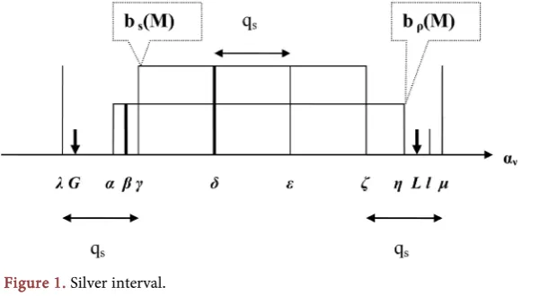
In the below Figure 1 we see that the band b Ms

( )

=

[

γ ζ,

]

has a “length”

3

M s

d = q _{and not} dM >4qs as the (4.5) implies above, however that was done

die to the simple supervision and obviously it will not interfere with the proving methodology that will be shown below. (A composite natural number is the one that is not prime). In general all the prime-multiples numbers of a random prime number qs (meaning all its integer multiples, that were named qs-multiple

numbers) function as erasers in the list of prim number candidates, since they erase the possibility of being the natural numbers with which the prime numbers coin-cide. Using this interpretation they will be named qs-multiples erasers. These are

the ones that the tracker changes their color from light blue to black (erasure) as soon as the tracker meets the first qs number on the unending travel of the

axis aν =ν of natural numbers.

In Figure 1 are shown the two boarders 2

M

G q= _and 2 1 1

M

L q= + − of the

random silver interval 2 2

)

1

, M q qM M

δ _{= } ₊ _where: 2

1

1 _M 1

L l= − =q + − (4.6)

Also in that same figure are seen the two bands b M_s

( )

=

[ ]

γ ζ, _of q_s and the b Mρ

( )

=

[

α η,

]

of qρ. Where λ, , , , , , , , , , ,Gα β γ δ ε ζ η L l µ obviously

[image:13.595.228.529.562.727.2]

natural numbers on the axis of natural numbers aν. The band b Ms

( )

with geometrical length nqs and n = 3 for Figure 1, will include n + 1 multitude of

(14)

s

q -multiples erasers that is Figure 1 are the

γ δ ε ζ

, , , with properties:

s q

γ λ δ γ ε δ ζ ε µ ζ− = − = − = − = − = _{. In addition,}_β_{is a random}qρ-multiple

number of another random band b Mρ

( )

that as shown in the figure happens

to be overlapping with b Ms

( )

. The relation (2.1) shown in Section 2:

( )

1

1 1 1 1 1

2 3 5 7

M j

j M

P M P F

q ν ν ν =        = = = −_ _ − _ − _ − _ _ − _     _{ } 

∏

 (4.7)

is based on the assumption that the density of qj-multiples erasers in the silver interval δM, where j=1,2,3, , M is:

1 1: j j j q q

ρ = = _(4.8)

Thus, the active multitude of qj-multiples erasers in δM, with “length” dM

will be: M j j d K q

= _(4.9)

Hence, the non-erased natural numbers in δM from the qj-multiples will have as active multitude

1 1 j M j F d q   = −_ _

  (4.10)

However, owing to two random bands b Ms

( )

and b Mρ

( )

of δM not

hav-ing the same boarders, as shown in Figure 1, meaning that theirs boarders do not coincide (i.e.

α γ ζ η

≠ , ≠ in Figure 1) the active multitude of the erasers of the assumption in δM will not coincide with the true multitude of erasers.

Let Ks the unknown multitude of qs-multiples of these erasers of δM. It

was shown before that all these numbers belong to b Ms

( )

of δM and are of

multitude n + 1 (with n = 3 in Figure 1). Hence, in general it will be true: 1

s

K = +n _(4.11)

However due to the relation (4.8), (4.9) and based on the help of Figure 1 in the general form it would be

(

) (

)

M s j M

s s s s s s

G l

d l G G l

K d n

q q q q q q

γ ζ

γ ζ γ ζ

ρ − − − − − + −

= = = = + + = +

The remainders between the silver interval δM and the band b Ms

( )

are the intervals

γ

−G_and l−ζ _{, that obviously each one of these is less or equal}

to qs not however both equal to qs, because then qs =qM =qM+1, which is

absurd, hence it is true that

(

) (

)

0 2

s

G l

q

γ− + −ζ

< <

Combining the last relation with the expression of Ks from above, it is given: 2

s

(15)

1 s s

K >K − (4.13) This relation (4.13) shows how the expected multitude of prime numbers in the δM interval will have to be as a whole greater than the true multitude, since

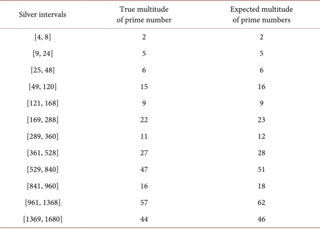
the active multitude of the erasers is generally smaller that their true multitude, fact that was confirmed using computer based calculations and will be further explained in the following analysis. In the table below is shown the changes be-tween the true and expected multitude of prim numbers in the first 12 silver in-tervals. The expected or active multitude of prime numbers is calculated using the relation QM =Int P M d

( )

⋅ M= Integral part of P M d

( )

⋅ M .

A random eraser, prime-multiple, of band b Ms

( )

, let that be δ, would have non-zero probability coinciding with another eraser qρ-multiple, let that be β,

of another band b Mρ

( )

(that is overlapping with band b Ms

( )

and β is not in the overlapping region) if the left boarders γ, α of b Ms

( )

and b Mρ

( )

were

coinciding. In this case [which is the implied acceptance of (2.1) or (4.7)] there is a possibility of the creation of an additional prime number, than it would in re-ality, because this way the capability of erasing of the eraser δ is cancelled, since it is degenerating into the erasing that is already fulfilled by the other prime-multiple eraser β. To reverse the possible redundancy by 1 of multitude of active erasers in comparison to the multitude of real, due to the boarders γ, α, not overlapping and instead to increase it, it is enough to increase Ks by 1. However, how would one explain the choice to increase “by 1”? The proof, for its necessity, is that if the left boarder γ, of a random band b Ms

( )

, was overlap-ping with the left boarder G of the silver interval of δM, then b Ms

( )

would include at most one more eraser x. It should be highlighted here that only this eraser introduced error (and thus causes the difference in active and real values), because this is the only one missing from the area Gγ <qs, resulting in the

sta-tistically expected cancelling of the erasing ability of another eraser of another band being included in the calculations of the relation (2.1)—only from this x—, due to the statistically expected overlapping of x, β in G

γ

_{. With this virtual}

cancelling will reasonably be born in the statistical calculations of (2.1) fewer prospective (active) erasers. This way, however, there will be, from (2.1), more prime numbers than the real ones, because x does not exist (i.e. virtual), hence it did not accomplish statistical erasing, like β did. So to reverse the result x needs to be added to become from virtual to real. The same will be true for the right boarder ζ of b Ms

( )

.

Similarly, because the right boarders e.g. ζ, η of b Ms

( )

, b Mρ

( )

are possibly,

in general, not overlapping, there needs to be anew an increase in the active multitude Ks, for the same reason as before, by one more unit. In total, by in-creasing Ks by 2, the new active multitude of erasers for b Ms

( )

will be for every case greater than the real multitude of Ks, owing to the fact that it is like

placing in each one of the two intervals [G,γ) and (ζ, L] one qj-multiple eraser, which is over-covering, because the λ, μ do not, as a rule, overlap with G, L re-spectively. Thus one concludes in the relation

, 2

s NEW s s

(16)

DOI: 10.4236/apm.2019.99038 809 Advances in Pure Mathematics More specifically, one can show (4.14) in a different way, shown below. If all the bands had, in the ideal case, their left and right boarders same as the borders G and L respectively of δM (Figure 1) then the easers would increase by

mul-titude 2M −2. The −2 is present because the b MM

( )

band of qM has

al-ready the same left boarder (limit) with G, but also another one, the b M1

( )

of

1 2

q = _{has the same right boarder with}_L_{. Splitting the multitude of the new}

erasers (that transform, the distribution of prime numbers qs in the δM

in-terval into an ideal one, and thus over-covering the error), in the band M of δM.

There will be an increment for every band of this ideal case [of (4.7)] by

(

2M−2

)

M = −2 2

(

M

)

<2. So with 2 further erasers, for every band, the over-covering mentioned before is certain. Because in this way a new ideal dis-tribution is born “that it is certain to realise all the missing erasing and even more”. That leads to an inequality.

A more analytical proof of the above is given here. Let µmk_m be the new in-creased (by 2) multitude of erasers of the band b mk_m

( )

, which is the band km

of δm silver interval. Let I=1QM be the definition of a new unit with

1 1

m

m m

T m M

M mk

m k

Q =

µ

= =

=

∏ ∏

. The new unit I (instead of the previous one which is 1)

subdivides now, to more parts the interval, that is defined by the subsequence of M of sequential silver intervals on the axis of natural numbers, with multitude

m

T ∈N of bands, the catholic selected among them δm. It is clear that every

unit of natural numbers, which is the distance 1 of two sequential natural num-bers on their axis, to the last silver interval δm, will be subdivided in multitudes

M

Q equal parts. Afterwards, the erasers of every band are equally distributed in every single silver interval. It is obvious that there will be created Μ multitude new virtual silver intervals that will have all their erasers qkm-multiples placed on the new marks that define the smaller according to the factor QM new

sub-divisions, where each subdivision has length I. So after the increment by 2 eras-ers of every band b mk

( )

and after equally distribution of erasers in all bands and in all these, M multitude, virtual silver intervals, we conclude that the eras-ers of every band b mk

( )

_{become more frequent and thus finally the previous} ability of distribution:

1 1 m

m m

M k

M k k

Q

Q q q

ρ

= ⋅ =

transforms in a new greater distribution density:

1 _m 1 _m

m

m m

M M k k

k

M k k

Q Q

Q q q

ξ ξ

ρ = ⋅ + = +

where according to the previous ones and because the increment for every band by 2 erasers; the following will be true:

2 _0, _, m

m

k m

k

k m

u

ξ

= > ∀ ∀

(17)

DOI: 10.4236/apm.2019.99038 810 Advances in Pure Mathematics erasers of the band b mkm

( )

. It becomes clear, on the one hand, that in every single virtual silver interval δm, due to the equal distribution of the erasers of

every band in it, it would now be true the exact corresponding relation of the previous (4.7) so as to estimate the prime numbers in every silver interval δm.

That means that now the ideal—for the precise calculations of the multitude of prime numbers—new virtual density ρk_m (that will be used and directly below) is used instead of the real and non-ideal ρk_m that was used before in (4.7). On the other hand, it is realised that in this way there will be less virtual prim num-bers (in every δm), since there are more erasers for every band of every silver

interval δm. The index km obviously corresponds to the index s of δM for the

random now intermediate or non silver interval δm. Leaving the above boarder

M of the arbitrary elected sequence, of the successive silver intervals δm, to tend

towards infinity; all the different cases are covered. It is very important to em-phasize that this method of creating the virtual silver interval functions as fol-lows: “In order the true multitude of erasers to coincides with their active multi-tude, all erasers should belong to bands which would had their boundaries in common with the boundaries of their silver space δm, so that in this case, on the

one side the random band b Mj

( )

would had the predicted density 1qj of erasers, and on the other side this band would had equal distribution of all its erasers in its total δm. So in this case would be made the coincidences of erasers

predicted by the statistics of relationship (4.7), so that finally the relationship (4.7) would function correctly. But that does not happen. Therefore, with the virtual silver interval we achieve the equal distribution of the erasers of random band in the total δm, that is we achieve the realization of the statistically

pre-dicted coincidences from the relationship (4.7), and on the other hand simulta-neously we succeed that these erasers to have greater density than the real den-sity 1q_j. So finally in the virtual silver interval we will surely have more write-offs than the real ones. In others words we will have something that re-quired from the asking inequality”. This proof, combined with the definition of the virtual silver interval of precise calculations of prime numbers (due to the equal-distribution of the erasers of the bands as mentioned), will clarify the analysis below, of the inequalities mentioned and justified before, with a differ-ent additional way.

It is observed that in the relation (4.5) it was proved that dM >4qs. So now,

the two additional erasers of relation (4.14) must be distributed in more than 4

s

q -multiples of b Ms

( )

. [The band b Ms

( )

of Figure 1 has geometrical length 3 4

M s s

d = q < q , instead of dM >4qs, owing to the relation (4.5), however, this

is not inadequate, because as stated it was done only due to the simple impedi-ments and it clearly does not influence the probative methodology]. So, with this distribution that creates the new active multitude of its erasers (4.14) based on the old one, on every one of the old erasers there will be added at most 2/4 = 1/2 erasers. In more details from the relation (4.14) one gets: s 2 s

M M

K K

d d

+

(18)

DOI: 10.4236/apm.2019.99038 811 Advances in Pure Mathematics to the dM >4qs results in s ₄2 s

M s M

K K

d + q >d so

1 2

s s

s q

ρ + >ρ _{, and due to}

1

s s q

ρ = _{of (4.8) one results:}

1 1

consequent

2_, _1, _ly 1.75 1.75 7

2 8 s s s q q ρ ρ  

< ∀ > < = =

 



 (4.15)

So for the absolute validity of the inequalities (4.15) the fact that the active density ρ =s 1qs of every band b Ms

( )

[that is used in the relation (2.1) or (4.7)] was considered to probably be a bit greater, because every band (that is enclosed on its whole in the silver interval δM) does not include exactly n

mul-titude of qs-multiples erasers, as implied by the expression ρ =s 1qs, but

1 n

+

, which is explained using Figure 1. [For example ρ =s 1qs means that

( )

s

b M in Figure 1 will include 1 qs-multiple eraser in each one of these three

intervals [γ, δ), [δ, ε), [ε, ζ], that means 3 and not 4 of qs-multiples, that it

in-deed contains]. Therefore, in order to be led in the two relations (4.15) one is obligated to use the expressionρs=

(

n+1

) ( )

nqs =

[

1qs

]

+ 1

( )

nqs , instead of the relationρ =s 1qs . Additionally, because it was said dM >4qs,

n

>

4

will be

true [owing to the band b Ms

( )

necessarily includes all the qs-multiples of M

d ], so in every case there is ρ_s<5 4

( )

q_s _{. Thus, based on all the previous}

1.75 2

s qs qs

ρ < < _{will be true, which led to the two relations (4.15) that will}

be used below, because it was shown that they are generic and true for every case. On the grounds that, even if the observation ρ_s =

(

n+1

) ( )

nq_s _{is not taken into}

consideration and by simply accepting that ρ =s 1qs, then ρ <s 1.5qs <2 qs

will arise, which drive to the same conclusion that the above relation (4.15) is true. As a result the true probability will be defined respectively by (4.7) using the true density ρs which satisfies the relation (4.15), meaning:

( )

(

1

)(

2

)(

3

) (

)

1 1 1 1 1

M

j M

j

p ν Pν ν F ρ ρ ρ ρ

=

= =

∏

= − − −  − (4.16)

And now obviously due to the (4.15) it is true that:

( )

2

1 ₁ 2 _, 8

M

j j

p P M N

q

ν

=

 

= > _ − _ ∀ ∈

 

∏

(4.17)

However, in this way an interesting scenario occurs, a sequence of inequali-ties:

( )

2 1 1 1 1 1 1

1 1 ₁ 2 ₁ 2 ₁ 2 ₁ 2 ₁ 2 8 8 3 5 7 11

2 2 1 1 3 5 9 11 15

8 3 5 7 1113 17

2 3 2

1 1 3 5 7 8 9 11 13 14 15

8 3 5 7 8 9 1113 14 15 17 1 2

M j

j M

M M

M M M M

M M M

p P F

q

q q

q q q q

ν ν ν = − − − − − −       

= > = _ − _ − _ − _ − _ _ − _

    _{ }   − −  =       − − −    

> _ _ _ _ _ _

+ −

     

∏



 

1 1 , , 8

M

M M

M N

q ν δ

 

 

 

(19)

DOI: 10.4236/apm.2019.99038 812 Advances in Pure Mathematics Particularly, all the successive fractions of the type ν ν

(

+1

)

_{were inserted in}

brackets (…) exactly where they were missing, which creates a more enhanced inequality.

The last arose after the erasing of the equal numerators and denominators. Consequently for the true function p

( )

ν _{, that defines the exact number of prime}

numbers in the random silver interval δM, the result will be:

( )

1 1

8 M 8

P p P

q

ν ≥ ν = ν > ≥ _ν , ∀ ∈ν δM and

∀ ∈

M N

(4.18)

The last inequality from the tree inequalities of the relation (4.18) derives ob-viously from the relation 2 2

1

M M

q ≤ =ν αν <q + that defines the natural numbers

ν of the silver interval δM, whilst the first inequality (4.18) derives from

every-thing that was mentioned before for the consequences of the non-overlapping of the limits of b Ms

( )

and b Mρ

( )

, however this will not be used in this proof.

The inequality p

( )

ν >1 8

(

qM

)

of the relation (4.18) will be named fundatal inequality of the silver intervals. The inequalities (4.18) are these that as men-tioned will be proved in regards to the relation (2.1) when menmen-tioned in Section 3 that (2.1) along with everything that will be shown related to it below, includes all the available catholic information.

Previously, the probability p

( )

ν =P M

( )

=Pν was characterized as exact

func-tion meaning that it calculates the exact number of prime numbers in δM. The

function p

( )

ν , even unknown is said here to be exact in the sense that the in-equality (4.18) can be used for it, exactly like an inin-equality can be used for number π in the sense that in theory this number exists in any desirable precision. The proof of (2.1) is completed based in the independent divisibility of the prime numbers, like it was determined in Section 2. It is noticed that the fundamental inequality is the “function” of each silver interval, and this concept is a form of correcting (2.1) specifically for every silver interval, because the equal-distributions of prime numbers are disturbed in the limits of δM. Hence now, the wanted tally of the

events of twins (and maybe of other formed prime numbers) to infinity can be assessed whether it has a finite result or not.

Observing Table 1 the reason can be understood. The generator of prime-multiples numbers is, as explained in Section 3, an ideal mathematical generator that would define precisely the multitude of prime numbers in every single one of the silver intervals δM if the bands had the same limits, which is

shown by the procedure of calculation of the active probability

( )

p ν =P M =Pν in the proof of (2.1) [or (4.7)] that means one precise

calcu-lation based on the absolutely know tally of the prime-multiples natural numbers that consist a perfect repetitive procedure in every silver interval δM. If now (2.1) is

combined with the exact constraint of (4.17), that was shown it is understood that (4.17) is not refuted in any δM to infinity. An assessment, without essential

(20)

[image:20.595.210.538.89.324.2]

DOI: 10.4236/apm.2019.99038 813 Advances in Pure Mathematics Table 1. Prime multitude in silver intervals.

Silver intervals _{of prime number}True multitude Expected multitude _{of prime numbers}

[4, 8] 2 2

[9, 24] 5 5

[25, 48] 6 6

[49, 120] 15 16

[121, 168] 9 9

[169, 288] 22 23

[289, 360] 11 12

[361, 528] 27 28

[529, 840] 47 51

[841, 960] 16 18

[961, 1368] 57 62

[1369, 1680] 44 46

however g=2_{was chosen because that was the one that allowed the erasing of} sequential fractions, which at the end led to the proof of (4.18) that in turn proved to be sufficient for the calculation of the multitude of twin prime num-bers, as it will be shown.

It was proven before, that an increment of ideal erasers (active) of every band for a mean multitude

(

2M−2

)

M= −2 2

(

M

)

, will cause expected correction. Indeed, by calculating the mean increment-correction of each erasers, [one in every interval qs⇒1qs in (4.7) or (2.1)] for every band b Ms

( )

, approx-imately equal to:

(

)

(

)

(

2 2

)

1

2 2 2 2 1 ₁

s

M M s

M M

n

n _q ₊ _q _q

− −

∆ ≅ ≅

+ +_ − _

Once can set in (4.16) ρ_s = + ∆

(

1 n q_s

)

_s instead of ρ =s 1qs of (4.7) or (2.1).

Meaning

1 s_, _{1,2, ,} s

s n

s M

q

ρ = + ∆ =  (4.18a)

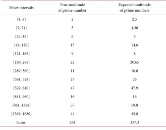
Based on this correction (4.16) forms the previous Table 1 as follows.

It is observed from Table 2 that there is indeed an important correction from an initial active multitude of 278 expected prime numbers, to 257.3 now. Mean-ing an error of approximately 1.4% from 6.5% that was before in Table 1.

(21)

[image:21.595.208.538.89.346.2]

DOI: 10.4236/apm.2019.99038 814 Advances in Pure Mathematics Table 2. Correction of prime multitude in silver intervals.

Silver intervals _{of prime number}True multitude Expected multitude _{of prime numbers}

[4, 8] 2 2.5

[9, 24] 5 4.36

[25, 48] 6 5

[49, 120] 15 14.6

[121, 168] 9 8

[169, 288] 22 20.65

[289, 360] 11 10.6

[361, 528] 27 26

[529, 840] 47 47.9

[841, 960] 16 16

[961, 1368] 57 58.8

[1369, 1680] 44 42.8

Sums: 264 257.3

(

₁

)

2

R= N− p (4.19) The precise relation (4.19) derives from the independency of repetitions in a multitude of Ν − 1 boarders among these.

The known theorem of prime numbers that dictates a logarithmic distribution

[1] [3] [6] is essentially a statistical theorem. To be exact, in this paper’s Statistics, based on the relations (2.1), (4.18) that were proven and will be utilized below, it will additionally be validated that “the catholic (random) selection of a prime number qa (that was named in the beginning of this paper) in an also catholic

(randomly) selected silver interval δM, does not give the catholic information

(that was also named in the beginning of this paper) that the probability of ap-pearance of the next prime number qb is changing in the very same silver

in-terval according to the distance of its position from qa”. The useful meaning of