Positioning in Dynamic Testing of Slender Bridges

(1)

Positioning in Dynamic Testing of Slender Bridges

Alexander Tesar1, Jan Bencat2

1

Institute of Construction and Architecture, Slovak Academy of Sciences, Bratislava, Slovak Republic; 2Department of Structural Mechanics, University of Zilina, Komenskeho, Zilina, Slovak Republic.

Email: [email protected], [email protected]

Received June 5th, 2011; revised July 6th, 2011; accepted July 18th, 2011.

ABSTRACT

The positioning combined with multi-functioning and interactive mechanics in dynamic testing of slender bridges are treated in present paper. The approach takes into account multiple functions in dynamic testing of slender bridges con-structed of thin-walled structural members with their hierarchical configuration. Theoretical, numerical and

experi-mental in situ assessments of the problem are presented. Some results of the application in situ are submitted.

Keywords: Bridges, Deformation Positioning, Dynamic Testing, Interactive Mechanics, Fourier Transformation, Multi

Functioning, Optimization, Virtual Monitoring, Wave Propagation

1. Introduction

One of interesting features of natural organisms from a design point of view is the co-existence of multiple func-tions in a single component. Natural organisms are the set-ups with many sub-systems being integrated together. The nature contains countless elegant and highly multi- functioning systems that are of great relevance to human design [1].

Such integration and multi-functioning appear also in dynamic testing and virtual monitoring of deformation positioning of slender bridges used in present structural engineering. Some previous studies of the problem are summed up, for example, in references [2,3]. During de-velopment of slender bridges the engineers have adopted a design philosophy of integrating various design functions together. Some of the issues considered in their design are mentioned as follows:

1.1. Multi-Function 1—Optimal Loading Control

The loads can be varied by suitable geometry and shape of structural members adopted. For example, the wind turbulences produce a strong vortex wake associated with aerodynamic drag force experienced by structural mem-ber. Depending on the wind speed and the cross-section’s shape, the shedding of vortices is more or less regular with shedding periods inversely proportional to the wind speed. In resonant conditions structure’s oscillations con-trol the rhythm of the vortex shedding appearing. Aside the known vortex trail type excitation the more general

types of aerodynamic forcing appear there. Aeroelastic forces proportional to the movement of the structure re-sult in self-induced vibrations at high wind speeds. In design is to be avoided that absolute value of negative aerodynamic damping force exceeds the positive me-chanical damping force producing oscillatory torsional or across-wind flexural mode instability.

1.2. Multi-Function 2—Optimal Structural Layout

The layout of structural members in slender bridge is optimal for generating an efficient flow of forces. Be-sides an optimal layout the bridges also have optimal material and shape properties being structurally efficient for resisting loads. The single member is in a continuous contact with other members and the modeling takes into account all interactions appearing.

1.3. Multi-Function 3—Optimal Fail-Safe Mechanisms

(2)

adjacent members before serious damages occur. Once unzipped the elements can be re-zipped together by sim-ple load and stress redistribution. The large number of separate zipping mechanisms ensures that the structure will unzip very close to the limit point of overload, thus causing minimum damage.

1.4. Multi-Function 4—Tuned Behaviour Control

New devices for tuned behavior control are also multi- functionally adopted in slender bridges. For example, to ensure the satisfactory interaction between such materials as fiber composites, wood, steel or concrete, the shear connectors have to be placed in the areas of concentrated load introduction. Such tuning facilities are adopted with regard to three main items as are the changes in stiffness, moment resistance and rotation capacity (ductility). Tuned vibration with control joints also contributes to multi- functioning in slender bridges subjected to vibration forcing.

Some approaches dealing with multi-functioning in dynamic testing and virtual monitoring of slender bridges are considered in this paper. Dynamic testing is applied to slender bridges as part of their inspection and assess-ment. Such technique is adopted with emphasis on data processing and experimental set-up involved in the evalua-tion of the dynamic amplificaevalua-tion factor and dynamic properties of the bridge. Vertical accelerations, displacements and strains are measured under ambient traffic. Such approaches are observed by experimental and ana-lytical studies in bridge dynamics (see references [2,3]). Most dynamic tests are carried out to evaluate dynamic properties (vibration frequencies and mode shapes, power spectral density, linear and nonlinear time response, etc.) using direct input force mechanisms (shakers, running trucks, impact testing) and modal analysis techniques. These properties are used for finite element model cali-bration and as a reference in monitoring of dynamic be-havior of bridge structures.

2. Structural Assessment

Primary point in structural assessment is the evaluation of the dynamic amplification parameter DAF generated by traffic loads on bridges. The parameter is specified by



1



dyn sta

R R DA (1)

where Rdyn is the maximum response of the bridge gener-ated by a moving load (maximum dynamic response) and

Rsta is the maximum response generated by the same load applied statically (maximum static response). The term (1 + DA) is called the dynamic amplification factor (DAF) and is the amount by which the static effects are in-creased by bridge-vehicle interaction. For design

pur-poses dynamic load allowance coefficient DLA is adopted, based on statistical values of DAF obtained by dynamic testing and analysis. This coefficient is usually related to first vibration frequency of the bridge or to its span length.

The analysis is based on the the presumption of propa-gating waves with efficient exchange of potential and kinetic energy appearing. The bridge is radiated by the waves initiated by traffic or other load impacts and the response appearing is transmitted into all structural parts studied.

The wave propagation has two physical aspects—the source of waves and the medium where the waves are running. The waves initiated in the source are filtered during propagation in the bridge and are specified by spectral evolution. The diffraction of waves appears there in the inhomogeneities of the bridge.

The spectral evolution is based on following defini-tions:

1) Each stationary function x(t) is interpreted in inte-gral form by

 

ei t d

x t    A

 

 (2)

with A() as orthogonal complex process and with fre-quency ω.

2) The linear transformation y(t) of the function x(t) is given by

 

e di t



Y t  H i  A 



(3)

with H(i) as admittance function and eiωt as unit im-pulse adopted.

3) The spectral densities Sx and Sy of functions x(t) and

y(t) are related by

 

2

y x

S  S   H i (4)

The structure is defined by wave numbers ri() with longitudinal and shear waves.

The stationary waves are emitted from the source with amplitude F(, zo), i.e., z = zo. The wave superposition is given by

 

_

, e i t eir z d ,

i o

w t z     F  z



(5) The structural inhomogeneity is touched by propagat-ing waves. The response spectrum for such case is given by







 



2 2 Im  

, 0 , , 0 e r

R o

S  S  z H   _ _

 (6)

Response spectrum obtained is the basis for specifica-tion of physical parameters in virtual monitoring of bridges, with adoption of the identification approach de-scribed below.

3. Identification Approach

(3)

k

processes ex(tk) and em(tk). Discrete time equivalents

x(tk+1) and y(tk+1) are given by

 

k 1

 

k ex

 

x t  F x t B t

    (7)

  

k 1 1 2



 

k em

 

k

y t G G A x t t

     (8)

where the state vector x contains the members related to the bridge with possible stochastic properties and so do the system matrices F, B, A, G1 and G2 (see references [4]

or [5]).

Covariance matrices for forcing are denoted Rx(ti) and

Rxm(ti). The covariance matrices Y(ti) of the process y(tk)

with system matrices of the model are given by

 

1

 

K i K

Y t GF M t i

i

(9)

with

 

T

 

i x i xm

M t FR t G BR t (10)

The Hankel matrix established by covariance matrices

Yk(ti) is used in identification and is given by operations: 1) Form the Hankel matrix of the problem studied. 2) Compute the singular value decomposition of the Hankel matrix by

 

2 T

H p  U T V (11)

where U and V are orthogonal matrices and T is diagonal and semidefinite matrix of singular values.

3) System matrices are given by

 

1 T

F _ T U H p V

(12)

T _n

M  T V E (13)

n

G  E U T (14)

with



0 0 0



n n

E  I    . (15)

4) Solve unsymmetric eigenvalue problem established from the (m × m)-upper left submatrix of the (n × n)- system matrix F.

5) Compute modal parameters from eigenvalues and modes obtained.

6) Repeat the operations from step 4 for increasing system submatrix.

Before application of identification approach the fil-tering of data is required. The type of filter applied de-pends on actual forcing conditions appearing.

4. Ultimate Response

The Fourier integral transformation combined with the FETM-aproach [6] is adopted for dynamic testing. Con-sidered is the load Pj(t) moving with velocity c on the bridge studied. The load is located in time t in nodes j = 1,

2,..., n. The response in node i is given by Xi(t) (i = 1, 2, ..., m). The symbol gij() specifies the spectral re-sponse function in node i due to input unit impulse eit. There holds

 

   

d

X t  g t P t t (16)

with vectors X(t) and P(t) of functions Xi(t) and Pi(t), respectively, and with g(t) as (m × m)-matrix of functions

gij(ω). The response is given by

 



Y

M  N  Mp 



(17)

where N(ω) is the transfer function of the bridge and

MY(ω) is ultimate transform of forcing function MP(ω). The function of structural response N(ω) defines spectral characteristics of the bridge and specifies amplitude and phase shift of the response related to the components of the forcing assumed.

The approach allows the consideration of all structural parameters appearing. In updated Lagrangian formula-tion of moformula-tion geometric nonlinearities are implemented into coordinate transformations of the microelement mesh used. The physical nonlinearities are analysed on the level of macroelement mesh adopted.

5. Structural Optimization

Optimization is adopted as a selection of testing parame-ters in monitoring of bridges (see references [7-11]). The selection of testing parameters is subjected to following constraints:

 Geometric constraints—minimum and maximum areas, dimensions and rigidities of thin-walled members adopted,

 Stress constraints—maximum allowable stress,

 Displacement constraints—minimum and maximum deformations, rotations and displacements,

 Resonance, stability and fatigue ultimate limits. Such items specify the regional constraints and can be applied for all loads occurring. They are represented by constraint hypersurfaces. Stress, deformations and reso-nance, stability or fatigue ultimate limits are nonlinear functions of testing variables adopted. The constraint hypersurfaces are nonlinear functions of such variables. If virtual testing point lies above constraint surfaces then stress or displacements in regional constraints are within specified limits.

The optimization is stated as follows: Find the geomet-ric testing variables Y and the cross-sectional design vari-ables X or Z (as other types of variables) given by objec-tive function



, ,



min

W F X Y Z  (18)

(4)

L U

X X X (19)

L U

Y  Y Y (20)

L U

Z  Z Z (21) stress constraints

L U

    (22) displacement constraints

L U

r  r r (23) resonance, stability and fatigue constraints

L U

    (24) where the superscripts L und U denote the lower and upper bounds, respectively. The terms , r and  are the vectors of stress, displacements and resonance, stability or fatigue limits adopted. Such limits are implicit func-tions of testing approach given by following steps:

1) Assume an initial structural geometry,

2) Optimize testing variables for given geometry by satisfying Equations (18)-(24),

3) Modify the variables,

4) Repeat the steps 2 and 3 until the results are ob-tained.

The number of testing variables is to be reduced by specifying all above parameters in terms of a small num-ber of independent variables. In order to reduce the number of testing variables is used a coarse grid in the space of geometric variables, so that only a small number of X, Y or Z values is to be considered. In order to opti-mize the X, Y and Z variables, one of known uncon-strained minimization techniques (see references [6,9-16]) is to be used.

6. Application

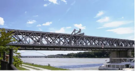
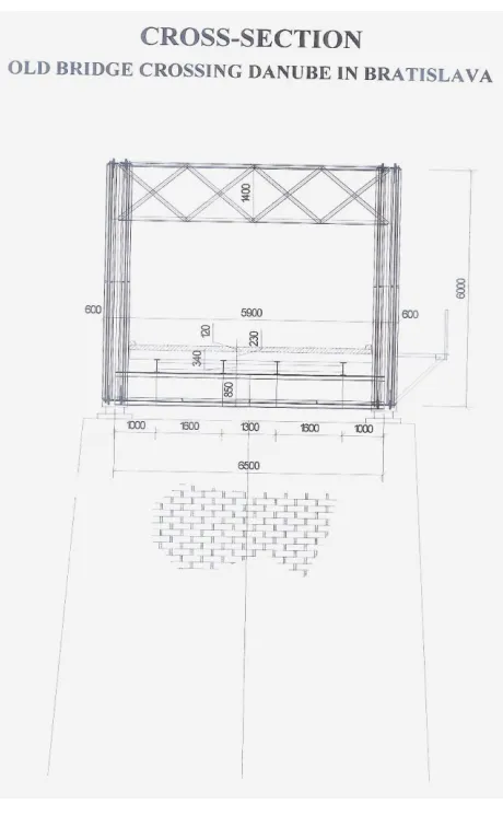
Studied is dynamic testing in monitoring of the Old Bridge crossing Danube in Bratislava, Slovakia ([4,5,17- 19]). The span of the bridge field studied is 75.82 m and

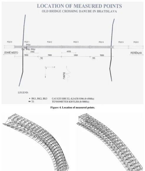
the width of the bridge is 7.00 m + 2.39 m (pedestrian path) (see Figures 1-4).

In scope of dynamic testing was studied the selection of testing parameters with following constraints:

· Geometric constraints, · Stress constraints,

· Displacement constraints—maximum midspan de-formation of the bridge was limited by 1/400 of the span,

· Resonance, stability and fatigue ultimate limits were assumed in accordance with valid standards.

The forcing was made by smooth runs of truck with weight 169.5 kN and with velocities 5 - 68 km/h.

Calculations were based on above theoretical approach and were confronted with experimental results in order to develop the model for the analysis. For calculation was adopted the software NASTRAN, with development of the models with optimal mesh in the FEM approach and taking into account actual boundary conditions of the bridge studied.

Calculated were 100 natural frequencies of vibration f(j)

with corresponding modal analysis and with determina-tion of corresponding 20 modes of natural vibradetermina-tion w(j).

[image:4.595.308.536.385.505.2]

The first 3 modes of vibration are plotted in Figures 5-7.

[image:4.595.55.543.552.707.2]

Figure 1. Studied span of the old bridge crossing Danube in Bratislava.

(5)

[image:5.595.57.287.81.454.2]

Figure 3. Cross-section of the bridge.

[image:5.595.303.538.102.446.2]

Corresponding natural frequencies are summed up in Table 1. The comparison of calculated and measured dynamic coefficients of the bridge at various truck veloci-ties is submitted in Table 2.

Significant goal was the assessment of actual stiffness of the bridge on the basis of calculated natural frequen-cies and logarithmic decrements of damping compared with corresponding actual values measured in situ.

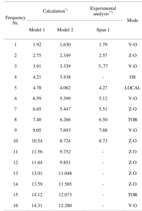
The frequency analysis submitted the information re-quired and was made in scope of all measurements done. Obtained were 112 spectra for specification of 9 domi-nant natural frequencies (3 for flexure in vertical direc-tion, 4 for flexure in horizontal direcdirec-tion, one torsional frequency and one frequency concerning the vibration of pedestrian path). The comparison calculation vs meas-urement for models without and with consideration of measured corrosion of the bridge is given in Table 3.

In Table 4 are summed up the dominant frequencies specified on the basis of the frequency analysis of the bridge. First frequencies in rows correspond to maximal

Table 1. Natural frequencies of the bridge.

Mode Natural frequency f(j) [Hz] Direction of vibration

1 1.630 Horizontal, flexure

2 2.349 Vertical, flexure

4 3.438 Horizontal, longitudinal

5 4.062 Local vibration

8 6.266 Torsion

15 12.073 Torsion

date in power spectrum SD(f)and the values in brackets represent frequencies with minor significance. In Table 3 is submitted also the comparison of natural frequencies found by numerical and experimental assessment.

Besides spectral analysis was made also the amplitude analysis submitting the basic stochastic parameters for the assessment. Statistical data obtained with 14 meas-urements on 4 channels submitted 504 values for ampli-tude analysis of the bridge. On the basis of extreme am-plitudes the dynamic coefficients δOBS were specified together with corresponding logarithmic decrements of damping. Evaluated were FFT-spectra (Fast Fourier Trans-formation) adopted for specification of 6 dominant fre-quencies as reference data in the assessment. Simultane-ously was made the spectral analysis for specification of coherence functions of the bridge. Some results are summed up in Figures 8-10 as well as in Tables 2 and 3. The damping coefficients of the bridge vary in scope 0.016 - 0.038. Amplitude analysis has submitted following maximal midspan deflections: 15.11 mm (flexure—vertical direction), 6.77 mm (flexure—horizonal direction)

(6)

[image:6.595.51.543.80.660.2] [image:6.595.56.290.451.685.2]

Figure 4. Location of measured points.

Figure 5. Old bridge in Bratislava—mode Nr. 1, f(1) = 1.630

Hz.

Figure 6. Old bridge in Bratislava—mode Nr. 2, f(2) =

[image:6.595.303.540.459.686.2]

(7)

[image:7.595.56.287.84.298.2]

Figure 7. Old bridge in Bratislava—mode Nr. 3, f(3) =

3.339 Hz.

Table 2. Dynamic coefficients of the bridge.

Old Bridge crossing Danube in Bratislava

Dynamic coefficient Smooth runs

1.span 1.span Run Nr. Direction V [km/h]

OBS (T1) EXP (T1)

1 BA-PE 8 1.096154 1.005865

2 PE-BA 9 1.244083 1.014889

3 BA-PE 18 1.239645 1.014618

4 PE-BA 18 1.553254 1.033749

5 BA-PE 27 2.337278 1.081574

6 PE-BA 27 1.254438 1.015521

7 BA-PE 34 1.366864 1.022379

8 PE-BA 39 1.627219 1.03826

9 BA-PE 54 3.017751 1.123083

10 PE-BA 45 2.736686 1.105938

11 BA-PE 54 2.988166 1.121278

12 PE-BA 54 2.233728 1.075257

13 BA-PE 45 2.899408 1.115864

14 PE-BA 68 2.943787 1.118571

All details concerning the calculations and measure-ments made (deflections, sensors, software, technical equip- ment, repeatability, etc.) are summed up in References [4,5].

7. Conclusions

[image:7.595.301.538.99.452.2]

Some approaches for dynamic testing of slender bridges are submitted. The procedures for dynamic testing were

Table 3. Comparison calculation vs measurement.

Calculation*) Experimental

analysis**)

Frequency Nr.

Model 1 Model 2 Span 1

Mode

1 1.92 1.630 1.79 V-O

2 2.75 2.349 2.57 Z-O

3 3.91 3.339 3.,77 V-O

4 4.21 3.438 - OS

5 4.78 4.062 4.27 LOCAL

6 6.59 5.399 5.12 V-O

7 6.65 5.447 5.51 Z-O

8 7.40 6.266 6.50 TOR

9 9.05 7.693 7.68 V-O

10 10.54 8.724 8.73 Z-O

11 11.56 9.752 - Z-O

12 11.64 9.851 - Z-O

13 13.01 11.048 - Z-O

14 13.59 11.585 - Z-O

15 14.12 12.073 - TOR

16 14.31 12.280 - V-O

*

FEM model 1—without considering of corrosion of load bearing members model 2—with consideration of corrosion (decrease of material 1 mm) and with dead weight of connecting members; **dominant frequencies with significant influence in spectral power density (PSD) data with non-significant energy influence in power spectral density.

LEGEND:

V-O—horizontal flexural vibration

Z-O—vertical flexural vibration

TOR—torsional vibration

OS—horizontal longitudinal vibration

applied in order to evaluate dynamic properties and cor-responding amplification factors. Such tests are part of bridge inspection in order to establish a basis for standard procedures in dynamic testing. Tests carried out under traffic on the bridges are preferred. Some results obtained are presented.

Specified were frequencies of vibration with modal analysis and with comparison of calculated and measured dynamic coefficients of the bridge studied. Significant was the assessment of the stiffness of the bridge on the basis of logarithmic decrements of damping compared with actual values measured in situ. Such analysis sub-mitted the information required and was made in scope

f all measurements done. Obtained were frequency o

[image:7.595.58.288.352.606.2]

(8)

[image:8.595.86.515.86.270.2] [image:8.595.81.520.301.490.2]

Figure 8. Time response of flexural deflection w(t) and power spectrum of response SD(f) in point BK1.

Figure 9. Time response of flexural deflection w(t) and power spectrum of response SD(f) in point BK2, smooth run Nr. 1, (BA

– PE), 1 × MAN, v = 8 km/h, wmax = 0.001581 m.

[image:8.595.82.515.531.707.2]

(9)

[image:9.595.60.286.137.437.2]

Table 4. Dominant frequencies of the bridge.

OLD BRIDGE CROSSING DANUBE IN BRATISLAVA

Smooth runs

Dominant frequencies [Hz] in direction Run

Nr. Direction Speed [km/h]

vertical (BK1) horizontal (BK2)

vertical

(BK3)

1 BA - PE 8 2.57

(0.878; 4.35)

2.57 (3.77; 4.35)

5.12 (2.58; 4.35)

2 PE - BA 9 _{(4.28, 5.81)}2.57 _{(3.77; 4.35)}2.57 _{(2.06; 5.12)}2.57

3 BA - PE 18 2.57

(1.33, 5.81)

2.57 (3.77; 4.35)

2.57 (1.65; 5.51)

4 PE - BA 18 _{(1.29; 2.57)}1.17 _(1.14;2.57)1.44 _(2.58;4.70)5.13

5 BA - PE 27 _{(2.57; 1.76)}1.16 _{(2.57; 4.35)}1.16 2.57 (1.16; _4.27)

6 PE - BA 27 2.57

(8.73; 5.12; 4.35) 4.35

(2.57; 35.12) 2.57 (0.33)

7 BA - PE 34 _{(1.16; 1.58)}2.57 _{(2.57; 5.14)}1.34 _{(5.14; 4.35)}2.57

8 PE - BA 39 2.57

(3.02; 8.5; 5.12)

2.57 (1.15; 4.14)

2.57 (4.70;5.12)

9 BA - PE 54 1.99

(1.15;2.57)

1.79 (1.15; 2.57)

2.57 (1.15; 4.71)

10 PE - BA 45 2.57 (4.14; 6.66) 2.57 (4.14; 6.66)

2.57 (5.12)

11 BA - PE 54 2.57

(1.99; 3.0 )

5.12 (2.57; )

2.57 (6.69; 4.66)

12 PE - BA 54 _{(2.57;3.03 )}2.30 _{(1.83; 4.24)}2.57 _{(2.57; 6.50)}5.13

13 BA - PE 45 2.57

(1.83; 2.99 )

2.57 (1.83; 4.24)

0.867 (2.57; 6.50)

14 PE - BA 64 _{(1.57; 2.03 )}1.39 1.31 (1.58; _1.80) _{(1.85; 2.57)}1.21

spectra for specification of dominant natural frequencies for flexure in vertical and horizontal direction as well as in torsion. The comparison calculation vs measurement was made without and with consideration of corrosion damages.

In addition spectral analysis was made in order to ob-tain stochastic parameters for the assessment. The spec-tral analysis was used for specification of coherence functions of the bridge.

All above parameters were adopted in approach de-veloped for dynamic testing and assessment of bridges.

8. Acknowledgements

Authors are indebted to the Slovak Scientific Agency VEGA for suggesting and supporting of above research in scope of scientific grants submitted.

REFERENCES

[1] L. Da Vinci, “Manuscript RL 19115v; K/P 114r,” Royal Library, Windsor Castle, Windsor, ca. 1500.

[2] P. Paultre, O. Challal and J. Proux, “Bridge Dynamics and Dynamic Amplification Factors – A Review of

Ana-lytical and Experimental Findings,” Canadian Journal of

Civil Engineering, Vol. 19, No. 2, 1992, pp. 260-278. doi:10.1139/l92-032

[3] J. Proulx, D. Hébert and P. Poultre, “Dynamic bridge testing in Quebec,” Proceedings of International

Confer-ence Structural Dynamics—EURODYN’93, Trondheim,

Vol. 2, 1993, pp. 943-950.

[4] J. Bencat, “Dynamic Testing of the Old Bridge Crossing Danube in Bratislava,” Technical Report Nr. 6-3-21/SvF/06, TU Zilina, 2008.

[5] A. Tesar, “Testing of the Old Bridge Crossing Danube in Bratislava,” Technical Report, 2001.

[6] A. Tesar, “Transfer Matrix Method,” Kluwer Academic Publishers, Dordrecht/Boston/London, 1988.

[7] R. Razani, “Behaviour of Fully Stressed Design of Struc-tures and Its Relationship to Minimum-Weight Design,” Journal Amer. Inst. Aeron. Astron., Vol. 3, 1965, pp. 2262-2268.

[8] R. L. Fox, “Optimization Methods for Engineering De-sign,” Addison-Wesley Publishing Group, Reading, 1971 [9] U. Kirsch, “Synthesis of Structural Geometry Using Ap-proximate Concepts,” Composite Structures, Vol. 15, 1982, pp. 103-111.

[10] L. A. Schmit and H. Miura, “A New Structural Analy-sis/Synthesis Capability—Access,” American Institute of

Aeronautics and Astronautics Journal, Vol. 14, No. 5, 1975, pp. 661-671.

[11] A. Tesar, “Synthesis in Optimisation of Shell Bridge Structures,” Building Research Journal, Vol. 35, 1985, pp. 812-824.

[12] J. Rechenberg, “Evolutionsstrategie,” Reihe Problemata 15, F. Frommann Verlag, Stuttgart, 1977.

[13] A. Tesar, “Load-Bearing Control of Slender Bridges,”

International Journal for Numerical Methods in Engi-neering, Vol. 62, No. 7, 2005, pp. 924-936.

doi:10.1002/nme.1213

[14] A. Tesar, et al., “Ultimate Response of Bionics Shells,”

Structural Engineering and Mechanics, Vol. 14, No. 2, 2002, pp. 135-150.

[15] A. Tesar, “Bionics and Fractal Configurations in Struc-tural Engineering,” International Journal for Numerical Methods in Engineering, Vol. 68, No. 7, 2006, pp. 790- 807. doi:10.1002/nme.1734

[16] S. C. Burgess, “Multi-Functioning and Multi-Optimization in Feathers,” International Journal of Design & Nature, Vol. 1, No. 1, 2007, pp. 1-10.

[17] J. Bencat, “Dynamic Testing of the Old Bridge Crossing Danube in Bratislava,” Technical Report Nr. 6-3/SvF/06, TU Zilina, 2006.

[18] J. Bendat and A. Piersol, “Engineering Applications of Correlation and Spectral Analysis,” John Wiley and Sons, Inc., New York, 1980.