Online Full Text

Abstract—This paper presents a quantitative analysis of the resolvable representation problem. I use a divide-and-conquer approach to allocate drawings to various categories based on readily-perceived characteristics of 3D objects, and generate a resolution sequence which takes account of these characteristics. The results suggest that most objects fall into categories for which optimal resolution solutions are readily identified and thus the resolvable representation problem can usually be avoided in practice.

Index Terms—Beautification, Resolvable Representation, Resolution Sequences

I. INTRODUCTION

In this paper, I analyse the problem of resolvable representationsof polyhedra, as first discussed by Sugihara [3]. This problem is of theoretical importance in constructive geometry and of practical importance in boundary representation CAD modelling. It is of relevance both in the field of automated interpretation of line drawings and the field of beautification of solid models (a subproblem of reverse engineering).

The resolvable representation problem is that of creating a

resolution sequence: given that we know the topology of a polyhedron, we wish to define its geometry by sequentially defining the coordinates of single topological items in such a way that, by the end of the sequence, the geometry of every topological item is defined, while ensuring that the overall geometry is consistent and free from contradictions.

This paper does not consider other aspects of geometric beautification. For a good overview of the state of the art, see Zou and Lee [8], which also proposes a solution to one of the other important and difficult subproblems, that of numerical redundancy in constraints.

Sugihara’s initial paper [3] on the resolvable representation problem considered only faces and vertices. He proved that all genus-zero polyhedra have resolvable representations, and outlined a general approach for finding them. Sugihara also showed by example that some non-genus-zero polyhedra have no resolvable representations if only faces and vertices are considered.

Sugihara gives, as an example of a polyhedron with no

Peter Varley is with the Department of Mechanical Engineering and Construction, Universitat Jaume I, Castellón de la Plana, Spain. E-mail: [email protected]

This work was funded by financial support from the Ramon y Cajal Scholarship Programme.

resolution sequence, the torus in Figure 1. Each face is a quadrilateral, and each vertex lies on four faces. Since vertex coordinates become fixed when three faces which touch the vertex are fixed, and face planes become fixed when three vertices which lie on the face are fixed, the last piece of topology in the resolution sequence can be neither a face nor a vertex. Ergo, no resolution sequence exists.

Figure 1: Sugihara’s Torus [3]

This paper addresses a point which Sugihara does not consider: in many cases, finding a valid resolution sequence is not the whole of the problem. There are other geometrical constraints on faces and vertices, and we generally wish to enforce an optimal subset of these. The problem then becomes that of finding a strategy which, firstly, enforces desirable geometric constraints, while, secondly, remains a valid resolution sequence. Section II discusses this in more detail.

In the knowledge that some objects have no resolution sequence, I do not seek a general solution. Instead, I present a divide-and-conquer approach based mainly on identifying desirable geometric constraints (principally parallelism and perpendicularity) and choosing an appropriate construction strategy which allows selection of a valid resolution sequence which enforces these constraints. This divide-and-conquer approach is described in Section III. Historically, divide-and-conquer has been applied successfully in geometric beautification ([4] is one such approach), for the purpose of creating the “most beautiful” interpretation of the drawing, but generally only in the context of trihedral objects, for which there is no resolvable representation problem.

The primary benefit of the divide-and-conquer approach is that the divisions correspond to the impression of the whole object formed in the mind of a viewer, who readily perceives objects as belonging to such types as normalons, quasi-normalons and pyramids. Basing the division on such categories leads to methods which are intuitively correct in that they create the object a viewer would imagine when seeing the drawing.

A secondary benefit of this divide-and-conquer approach is that, for many of the resulting categories, the number of geometric degrees of freedom of the object can be determined

Resolution Sequences for

Geometric Beautification

exactly. The geometric degrees of freedom problem is another open problem in line drawing interpretation and beautification of solid objects which has no known general solution.

Degrees of freedom are important to the beautification process since most existing systems determine optimal geometry using some form of downhill optimisation. The number of degrees of freedom corresponds to the number of variables to be optimised. In general, the fewer degrees of freedom we have, the better, as fewer variables should lead not only to better results but also to faster running times.

II. DISCUSSION

There are a number of points to be considered concerning Sugihara’s initial paper on resolvable representations.

Firstly, it only considered faces and vertices. Edges are also an important part of topology—indeed, some topological categories, such as quasi-normalon, are defined by their edge structure—and must be considered too.

Secondly, Sugihara assumes that face equations are a single entity. In practice, it may be preferable fix face normals and face distances separately. One example of this might be when processing normalons: it is important to enforce perpendicularity on face normals very early in the proceedings in order to ensure that the resulting object is indeed a normalon, while retaining flexibility about face distances.

Thirdly, most objects will have several acceptable resolution sequences, and selecting one using a graph-based algorithm which does not consider other cues provided by the topology may well be suboptimal. What is required is, in general, a strategy (e.g. normals first for trihedral objects, vertices first for triangulated models), not a specific construction sequence.

Consider, for example, quasi-normalons. The ideal strategy would be to fix axis-aligned faces first, then vertices, then non-axis-aligned faces. However, we also need to make sure that we do not box ourselves into a corner unnecessarily: while a sequence exists, we must not fix anything which leaves us with no resolution sequence. Finding such an ideal strategy is a harder problem than the one Sugihara considers.

III. DIVIDE-AND-CONQUER

This section lists, in approximate descending order of frequency, groups of objects which have something readily perceivable in common. For “divide and conquer” to be worthwhile, we must identify divisions which are (a) easily identified, (b) easily conquered and (c) big enough to be worth conquering.

In all cases but the simplest, the divisions require additional knowledge beyond that of the object topology. This paper notes when additional knowledge is required, but does not consider its source (some knowledge can be deduced automatically, while otherknowledge may need to be entered manually).

Note that Sections IIIA (triangulated mesh models) and IIIB (trihedral objects) summarise work which can be found in most standard references. They are included for

completeness. The original content of this paper starts with Section IIIC.

In order to obtain an initial estimate of how common various categories of object are, I compiled a collection of approximately 1000 drawings of manifold polyhedra. Of these, 380 were neither fully trihedral nor triangulated mesh models.

A. Triangulated Mesh Models

A triangulated mesh is a polyhedron all of the faces of which are triangular. Triangulated meshes are comparatively uncommon in engineering objects, but extremely common in computer graphics applications since they are particularly easy to render, and also quite common in reverse engineering, where clouds of scanned points are usually converted into triangular nets.

Identifying triangulated mesh models is straightforward and can in principle be done in O(F) time: an object is a triangulated mesh model if each face meets exactly three vertices. No additional knowledge is required beyond the object topology.

There is a simple strategy for creating geometry for triangulated mesh models: (a) fix all vertex coordinates; and (b) calculate face equations by fitting a plane through the three vertices which lie on it.

All vertices in a triangulated mesh model can be moved independently, so have three degrees of freedom, so the total number of degrees of freedom of the object is 3V. Of these, 6 leave the object’s internal relationships unchanged: 3 translations, 2 rotations and 1 expansion/contraction. For example, the simplest triangulated mesh model, the tetrahedron, has 12 degrees of freedom, 6 of which can be used to distort the object.

B. Trihedral Objects

A trihedral object is a polyhedron all of the vertices of which are trihedral. Trihedral objects are comparatively common in engineering objects (for example, all extrusions of polygonal profiles are trihedral), and some sketching interfaces make the (useful but unjustifiable) assumption that

all engineering objects are trihedral.

Identifying trihedral objects is straightforward and can in principle be done in O(V) time: an object is trihedral if exactly three faces meet each vertex. No additional knowledge is required beyond the object topology.

There is a simple strategy for creating geometry for trihedral objects: (a) fix all face normals; (b) fix all face distances; and (c) calculate vertex coordinates by determining the point of intersection of the three faces on which the vertex lies.

Note, however, that although this strategy is valid, it is often not best. Many trihedral objects are also normalons (Section IIIC) or quasi-normalons (Section IIID), and the strategies proposed below lead to better (more “beautiful”) geometry.

change the object: 3 translations, 2 rotations and 1 expansion/contraction. For example, the simplest trihedral object, the tetrahedron, is its own dual, and has 12 degrees of freedom, 6 of which can be used to distort the object, regardless of whether it is processed as a triangulated mesh or as a trihedral object.

Where the object can be processed as a normalon or quasi-normalon, the number of degrees of freedom will generally be lower.

C. %on-trihedral %ormalons

Normalons are defined as those polyhedra in which all edges are aligned with one of three mutually-perpendicular axes. Many, but far from all, normalons are trihedral. The objects in Figure 2 are non-trihedral normalons.

Figure 2: %ormalons

Although the obvious normalon strategy (fix face normals first, then face distances) breaks Sugihara’s rules as originally formulated (i.e. each face is considered to be a distinct topological item) by fixing a non-trihedral vertex after the faces it meets, there is in reality no problem provided that coplanar faces are grouped together as a single topological item in the sequence. For example, although the central vertex in the left-hand drawing meets six faces, its geometry is defined by the intersection of three groups of coplanar faces.

27 objects from our test set are in this category.

Identifying such objects is straightforward and can be done in O(E) time: check that each edge is aligned with one of the main object axes. This requires the additional knowledge of which edges are axis-aligned. Axis alignment of edges from object topology and inexact geometry is one of the simpler things to determine automatically. It is generally reliable but can occasionally fail [5].

The construction strategy is: (a) calculate vectors for the three object-relative major axes, and apply them to all face normals; (b) fix the distance for each independent face (faces are independent unless they are demonstrably coplanar—for example, parallel faces which include the same vertex—in which case one face distance is fixed and applied to both faces); (c) calculate the coordinates of vertices by intersecting the face planes of the faces they meet.

The number of degrees of freedom is 3 for the orthogonal axis system plus one (the face distance) for each independent face. Again, 6 do not change the object: 3 translations, 2 rotations and 1 expansion/contraction. For example, the arrangement of four cuboids in the left-hand drawing has 9 independent faces so a total of 12 degrees of freedom, of which 6 distort the object by changing the relative proportions of the cuboids.

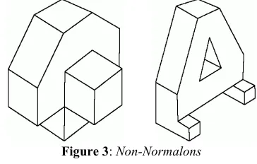
The same methods could in principle also be applied to

objects which are not normalons but where the non-trihedral part of the object is normalon-like, such as those in Figure 3. A further 3 objects from our test set are in this category. However, although the methods of this section suggest a preferred resolution sequence, the degrees of freedom calculation of this section does not apply. Rather than treat them as a separate category, it seems best to include them with the objects of Section IIIE.

Figure 3: %on-%ormalons

D. Quasi-%ormalons

Quasi-normalons are defined as those polyhedra in which all vertices lie on a graph-connected axis-aligned frame of edges. The objects in Figure 4 are quasi-normalons.

Figure 4: Quasi-%ormalons

The strategy here is (a) fix axis-aligned face normals and distances; (b) fix vertices; (c) derive face normal and distance for non-axis-aligned face(s) from the vertices which lie on them.

In the right-hand drawing, this approach corresponds to Sugihara’s rules, as the non-axis-aligned face is triangular.

The left-hand drawing illustrates an important point. We know that the four-vertex non-aligned face is planar in principle because all of the vertices lie on one of two parallel edges. Fitting a face to vertices which lie on one of two parallel edges is clearly a legitimate thing to do, and a technique which we can make use of in other categories of object. Even though we are breaking Sugihara’s rules by first calculating the coordinates of four vertices and then calculating the face equation of the face they lie on (because of roundoff error, calculating the face equations in this way will not necessarily result in all four vertices lying exactly on the face), this it is still the right thing to do, as it corresponds to the way we intuitively create a mental construct of the object when we view the drawing.

such objects is exaggerated, they occur frequently and it is important that they are processed correctly.

Identifying quasi-normalons is in principle straightforward: list all axis-aligned edges and check whether or not they can be connected to form a single graph. This is the graph connectivity problem, known to be soluble in linear time. As before, this requires additional knowledge: which edges are axis-aligned.

The strategy for processing quasi-normalons is: (a) calculate vectors for the three object-relative major axes, and apply them to all axis-aligned face normals; (b) determine the face distances of all axis-aligned faces (note that, as in Section IIIC, some faces meeting at non-trihedral vertices may be coplanar); (c) calculate the coordinates of vertices which meet three axis-aligned faces by intersecting the face planes; (d) fix the coordinates of any remaining vertices, while ensuring that they lie on the planes of any axis-aligned faces which they meet; (e) determine the equations of any remaining faces (triangular faces by fitting a plane through vertices, other faces by fitting a plane through two parallel edges).

The number of degrees of freedom can be obtained by considering the axis-aligned edges. In cases where all axis-aligned edges join two axis-aligned faces, such as the sliced cube in the right-hand figure, the number of degrees of freedom is the same as that of the normalon bounding box (in this example, 12, of which 6 do not distort the object).

However, where one or more of the axis-aligned edges bounds a non-axis-aligned face, more information is needed. The two such edges in the bracket in the left-hand figure illustrate this: the top is fully-constrained by the normalon bounding box, and adds no extra degrees of freedom, but the front edge can slide up and down without changing the character of the object, thus adding an extra degree of freedom.

Thus the total number of degrees of freedom is: 3 for the orthogonal axis system; one (the face distance) for each independent axis-aligned face; plus 0, 1 or 2 for each axis-aligned edge which bounds a non-axis-aligned face, depending on how fully the edge geometry is constrained by the normalon geometry. For example, the bracket has 11 degrees of freedom, of which 5 do not distort the object.

E. Resolvable as Quasi-%ormalons

In this section we consider objects which do not have a graph-connected quasi-normalon frame but for which the suggested quasi-normalon resolution sequence is the most appropriate. The objects in Figure 5 are resolvable as quasi-normalons (as were the objects in Figure 3).

Figure 5: Resolvable as Quasi-%ormalons

In the middle drawing, all of the non-normalon faces are triangular, so these can be placed last in the resolution

sequence. In the left-hand drawing, all of the non-normalon faces are either triangular or quadrilaterals defined by two parallel edges, so (provided that the disconnected edge is included in the resolution sequence) these again can be placed last in the resolution sequence. In the right-hand drawing, the quasi-normalon frame is not graph-connected but identifying axis-aligned edges remains straightforward.

Since this category of object lacks a formal definition, identifying which drawings fall into this category is not straightforward. Since the category is defined solely by the strategy, categorisation should proceed by determining what does, and what does not, cause problems for the strategy.

Faces with axis-aligned normals are unproblematic. Faces bounded by any pair of (implicitly parallel) axis-aligned edges are unproblematic provided that those edges are non-collinear. Triangular faces are unproblematic. Any face which is none of these is problematic, and any object containing such a face should not be included in this category.

The strategy for processing this category of object is the same as that for quasi-normalons (Section IIID).

The total number of degrees of freedom is even more complex than in the previous category, as each edge subgraph must be considered separately, as must isolated vertices such as the one in the central drawing.

Thus the total number of degrees of freedom is: 3 for the orthogonal axis system; one (the face distance) for each independent axis-aligned face; plus 0, 1, 2 or 3 for each axis-aligned edge which bounds a non-axis-aligned face, depending on how fully the edge geometry is constrained by the normalon geometry; plus 3 for each isolated vertex.

35 objects from our test set are in this category.

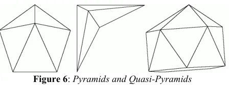
F. Pyramids

Strictly, a pyramid is a polyhedron which comprises a single base face and a single vertex, the apex, which does not lie on the base face and is connected by an edge to every vertex on the base face. The left and centre objects in Figure 6 are pyramids. Pragmatically, it is sensible to group together as a single category all polyhedra with only one non-triangular face. All pyramids fall into this category, and so does the quasi-pyramid on the right of Figure 6.

Figure 6: Pyramids and Quasi-Pyramids

The resolution sequence is straightforward: first fix the base face (normal and distance), then the vertices (in any order), and finally the triangular faces.

19 objects from our test set are in this category.

Identifying such objects is straightforward and can in principle be done in O(F) time: count the number of faces which meet more than three vertices. This requires no additional knowledge beyond the object topology.

objects: (a) fix the base face (normal and distances); (b) fix the coordinates of all of the vertices (ensuring that those vertices meeting the base face lie on the face plane); and (c) calculate the equations of each remaining triangular face by fitting a plane through the three vertices which lie on it.

The base face has 3 degrees of freedom. Each vertex meeting the base face must lie on the face plane, so has 2 degrees of freedom. Other vertices can be moved independently, so have three degrees of freedom. For example, the pentagonal pyramid on the left of the figure has 16 degrees of freedom, 10 of which can be used to distort the object.

G. Quasi-Trihedral Objects

We define quasi-trihedral objects as those objects in which no vertex meets more than three non-triangular faces. Figure 7 shows three such objects.

Figure 7: Quasi-Trihedral Objects

35 objects from our test set are in this category (the count does not include objects in previous categories—many quasi-normalon objects are also in this category, but not counted as such because processing them as quasi-normalons in order to preserve axis-alignment is more “beautiful”).

Identifying such objects is straightforward and can in principle be done in O(V) time: check the faces which meet each vertex, and ensure that no more than three of them are non-triangular. This requires no additional knowledge beyond the object topology.

The resolution strategy is straightforward: (a) fix the equations (normals and distances) of the non-triangular faces (some care is required here in order to ensure that this produces a valid sequence); (b) calculate the coordinates of all vertices (by intersection if the vertex lies on three known faces, otherwise fix any remaining degrees of freedom while ensuring that the vertex lies on appropriate faces), and (c) calculate the equations of the triangular faces by fitting planes through the vertices which they meet.

The number of degrees of freedom is: (a) each non-triangular face has 3 degrees of freedom; and (b) vertices have 3-N degrees of freedom, where N is the number of non-triangular faces meeting the vertex. For example, the rhombicuboctahedron on the left of the figure has 18 non-triangular faces so 54 degrees of freedom, 48 of which can be used to distort the object (this makes no assumptions about symmetry or axis-alignment, and a more beautiful result with only 30 degrees of freedom could be obtained by processing it as dissimilar parallel sections, Section IIII).

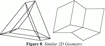
H. Similar Parallel Sections

Some objects, such as those in Figure 8, are created from similar 2D geometry on parallel planes. This includes objects

which are produced by the skinning or parallel section sweep

operations provided by many 3D CAD applications (the right-hand drawing in Figure 8 is one such), and also some objects which cannot be produced by these operations (for example, the left-hand drawing of Figure 8).

Note that, without the assumption that the three planes are parallel, the left-hand drawing (Sugihara’s Torus) has no construction sequence and the right-hand drawing must be processed using the general-case methods described in Section IIIJ.

Figure 8: Similar 2D Geometry

The construction sequence here is to create “ghost” faces for the three parallel planes. Using this as scaffolding, we can fix vertex coordinates and then create real faces from the “vertices on two parallel edges” rule used above.

9 objects from our test set are in this category.

Identification of these objects requires that object planes have been determined in advance (note that automatic detection of object planes from topology and inexact geometry is straightforward in principle but not fully reliable—see, for example, [7]). Identification of which vertices lie in which planes is then straightforward and can be done in O(V) time. Comparing the contents of the planes is the planar graph isomorphism problem, which has linear-time solutions (e.g. [2]).

The resolution sequence is: (a) fix a single face normal for the “ghost” faces; (b) fix the face distances for the “ghost” faces; (c) fix the coordinates for vertices lying on one of the “ghost” faces; (d) fix the offset and magnitude for each other “ghost” face; and (e) calculate the coordinates of the remaining vertices.

The number of degrees of freedom is: 2 for the ghost face normal, plus 1 for each ghost face distance; 2 for each vertex lying on the first ghost face; plus 1 for magnitude and 2 for offset (0 if the ghost face centres are aligned along the ghost face normal, which is most “beautiful”) for each remaining ghost face. In the case of Sugihara’s Torus, this gives a total of 13 for the “beautiful” version or 17 for the more general version.

In view of the limited number of objects in this category, and the fact that the method for identifying such objects is a subset of the method used to identify the next category, it might be preferable to combine the two categories.

I. Dissimilar Parallel Sections

The construction sequence here is to create “ghost” faces for the multiple parallel planes. Using this as scaffolding, we can fix vertex coordinates and then create real faces from the “vertices on two parallel edges” rule used above.

Figure 9: Dissimilar 2D Geometry

9 objects from our test set are in this category.

Identifying such objects is straightforward and can be done in O(V) time if the candidate plane orientation has been identified in advance: for each vertex, ensure that at least one of the edges is perpendicular to the plane normal. Note that this test is the same as the first part of the test for the objects in Section IIIH.

The resolution sequence is: (a) fix a single face normal for the parallel faces; (b) fix the face distances for the parallel faces; (c) fix the coordinates of all vertices, ensuring that they lie on the appropriate parallel face.

The number of degrees of freedom is: 2 for the ghost face normal, plus 1 for each ghost face distance; plus 2 for each vertex. For example, object in the left hand drawing, which has 16 vertices, would have 38 degrees of freedom. In principle, a significant further reduction in the number of degrees of freedom can be obtained in this case by noting that all of the faces on the parallel planes are co-oriented rectangles, but this is not an essential feature of the category. It is doubtful whether or not there are enough objects in this category to make it worth detecting. However, it is an obvious extension of the previous category. Since the method for identifying these objects is a subset of that used in Section IIIH, it might be preferable to combine the two categories.

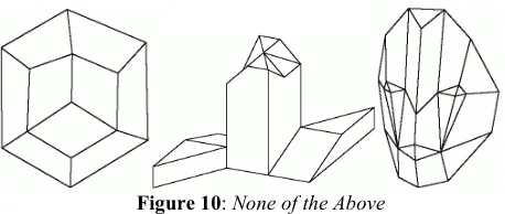
J. %one of the Above

A few objects fall into none of the above categories and remain a problem. Of our test set of approximately a thousand objects, only three fall into none of the above categories. These are the natural line drawings shown in Figure 10.

Figure 10: %one of the Above

These objects have nothing obvious in common with one another, other than that they are the source of a dilemma. In theory, all three are genus-zero objects, and, as Sugihara points out, a valid (but suboptimal) resolution sequence can be found using the Hopcroft-Tarjan algorithm [1] for trivalent decomposition of graphs. However, in practice, implementing the algorithm purely to cater for such a small group of objects

is undesirable, particularly since in each case a better solution is possible.

In the case of the left-hand drawing, the object geometry can be created from its threefold rotational symmetry (but not as a hexagonal frustum topped by a pyramid, which does not give a realisable geometry as the pyramid top must be in the plane of the frustum top). The middle object has twofold rotational symmetry, and the right object has mirror symmetry.

The practical dilemma is that, even though it leads to better results, implementing twofold, threefold and mirror symmetry categories for such small groups of objects (one each!) is also an ineffective use of resources. There seems to be no ideal answer.

IV. CONCLUSION

The quantitative analysis in this paper suggests that the resolvable representation problem is not a problem in practice. Most objects fall into particular categories for which optimal solutions are readily identified. However, for a small group of objects (less than 1% of polyhedral engineering objects) which fall into no such category, the recommended general solution remains suboptimal.

In general, categorising objects is straightforward. However, identifying normalons (Section IIIC) and quasi-normalons (Section IIID) reliably requires that axis-aligned edges can be identified. Current methods for automating this are not fully reliable, and further work is needed. Improved methods for identifying parallel planes of vertices (Sections IIIH and IIII) would also be helpful.

When an object falls into several categories, it is usually the case that the most “beautiful” results are obtained by choosing the category which gives the lowest number of degrees of freedom.

REFERENCES

[1] J.E. Hopcroft and R.E. Tarjan, Dividing a Graph into Triconnected

Components, SIAM Journal of Computing 2(3), 135–158, 1973.

[2] J.E. Hopcroft and J.K. Wong, Linear Time Algorithm for Isomorphism

of Planar Graphs, in Proceedings, 6th Annual ACM Symposium on

Theory of Computing, 172--184, 1974.

[3] K. Sugihara. Resolvable Representations of Polyhedra. Discrete and Computational Geometry 21(2), 243–255, 1999.

[4] P.A.C. Varley and R.R. Martin, A System for Constructing Boundary

Representation Solid Models from a Two-Dimensional Sketch, in ed.

W. Wang and R.R. Martin, Proc. GMP 2000, 13–32, IEEE Press, 2000. [5] P.A.C. Varley, Automatic Creation of Boundary-Representation

Models from Single Line Drawings, PhD Thesis, University of Wales,

2003.

[6] P. Varley, H. Suzuki and R. R. Martin, Interpreting Line Drawing of Objects with K-Vertices, Proc. Geometric Modeling and Processing 2004, Eds. S.-M. Hu, H. Pottmann, 249-358, 2004. ISBN 0769520782.

[7] P. A. C. Varley, R. R. Martin and H. Suzuki, Progress in Detection of Axis-Aligned Planes to Aid in Interpreting Line Drawings of Engineering Objects, in ed. T. Igarashi and J. A. Jorge, Sketch-Based Interfaces and Modelling, Eurographics Symposium Proceedings, 99-108, 2005.