PID Controller Design with Guaranteed Stability Margin
for MIMO Systems
T. S. Chang and A. N. G¨undes¸
Abstract— Closed-loop stabilization with guaranteed stabil-ity margin using Proportional+Integral+Derivative (PID) con-trollers is investigated for a class of linear input multi-output plants. A sufficient condition for existence of such PID-controllers is derived. A systematic synthesis procedure to obtain such PID-controllers is presented with numerical examples.
Keywords–Simultaneous stabilization and tracking, PID
control, integral action, stability margin.
I. INTRODUCTION
Proportional+Integral+Derivative (PID) controllers are the
simplest integral-action controllers that achieve asymptotic
tracking of step-input references [1]. Although the simplicity
of PID-controllers is desirable due to easy implementation
and from a tuning point-of-view, it also presents a major
restriction that only certain classes of plants can be controlled
by using PID-controllers. Rigorous PID synthesis methods
based on modern control theory are explored recently in
e.g., [2], [3], [4], [5], [6]. Sufficient conditions for PID
stabilizability of multi-input multi-output (MIMO) plants
were given in [6] and several plant classes that admit
PID-controllers were identified.
The systematic controller design method given in [6]
allows freedom in several of the design parameters. Although
these parameters may be chosen appropriately to achieve
various performance goals, these issues were not explored.
The authors are with the Department of Electrical and Com-puter Engineering, University of California, Davis, CA 95616. (emails: [email protected], [email protected])
The goal of this paper is to study closed-loop
stabiliza-tion with guaranteed stability margins using PID-controllers.
A sufficient condition is presented for existence of
PID-controllers that stabilize linear, time-invariant, MIMO stable
plants, where the closed-loop poles are guaranteed to have
real-parts less than a pre-specified−h. A systematic design procedure is proposed and illustrated with several numerical
examples. The choice of the free parameters can be
opti-mized with a chosen cost function. Although stability margin
can be considered as an important performance measure,
there are other factors effecting the performance of the
system and hence, “good” choice for the design
parame-ters for overall performance is case-specific and cannot be
generalized.
The paper is organized as follows: Section II shows the
main result, where a sufficient condition for stabilizability
using a PID-controller with guaranteed stability margin is
given. Section III presents a systematic procedure to
synthe-size PID controllers and gives several illustrative examples.
Section IV gives a short discussion, concluding remarks and
some future directions.
II. MAIN RESULTS
Notation: Let CI,IR,IR+ denote complex, real, positive real numbers. The extended closed right-half complex plane
in S; In is the n×n identity matrix. The H∞-norm of M(s)∈ M(S) is M := sup
s∈∂Uσ¯(M(s)), where σ¯ is the maximum singular value and∂U is the boundary ofU. We drop (s) in transfer-matrices such as G(s) wherever this causes no confusion. We use coprime factorizations overS;
i.e., forG∈Rpny×nu,G=Y−1X denotes a
left-coprime-factorization (LCF), whereX, Y ∈ M(S),detY(∞)= 0.
Consider the linear time-invariant (LTI) MIMO
unity-feedback system Sys(G, C) shown in Fig. 1, where G ∈ Rpm×m is the plant’s transfer-function and C ∈ Rpm×m
is the controller’s transfer-function. Assume thatSys(G, C)
is well-posed, G and C have no unstable hidden-modes, and G ∈ Rpm×m is full (normal) rank. We consider the realizable form of proper PID-controllers given by (1),
where Kp, Ki, Kd∈IRm×m are the proportional, integral, derivative constants, respectively, andτ ∈IR+ [7]:
Cpid=Kp+Ki
s + Kd s
τ s+ 1 . (1)
For implementation, a (typically fast) pole is added to the
derivative term so thatCpid in (1) is proper. The integral-action in Cpid is present when Ki = 0. The subsets of PID-controllers obtained by setting one or two of the three
constants equal to zero are denoted as follows: (1) becomes a
PI-controllerCpi whenKd= 0, an ID-controllerCid when Kp = 0, a PD-controllerCpd when Ki = 0, a P-controller Cp when Kd = Ki = 0, an I-controller Ci when Kp =
Kd= 0, a D-controllerCd when Kp=Ki= 0.
Definition 2.1: a) Sys(G, C)is said to be stable iff the transfer-function from(r, v)to(y, w)is stable. b)C is said to stabilizeGiff C is proper andSys(G, C)is stable.
The problem addressed here is the following: Suppose
that h ∈ IR+ is a given constant. Can we find a PID-controllerCpid that stabilizes the systemSys(G, Cpid)with a guaranteed stability margin, i.e., with real parts of the
closed-loop poles of the systemSys(G, Cpid)less or equal to −h? It is clear that this goal is not achievable for some
plants. Furthermore, even when it is achievable, it may be
possible to place the closed-loop poles to the left of a
shifted-axis that goes through−honly for certainh∈IR+. We start our investigation of plant classes for which we can achieve
our goal by considering stable plants. The class of plants
under consideration, denoted byGh, is described as follows:
Let G ∈ Gh ⊂Sm×m, i.e., let the given plant be stable. Furthermore, letGhave no poles with real parts in[−h,0]. Assume that G(s) has no transmission-zeros (or blocking-zeros) at s = 0, i.e., G(0) is invertible (note that this condition is necessary for existence of PID-controllers with
nonzero integral-constant Ki [6]). The plant G may have transmission-zeros (or blocking-zeros) elsewhere in U but
not ats= 0. Now define
ˆ
s:=s+h, or s=: ˆs−h (2)
and
ˆ
G(ˆs) := G(ˆs−h) ; (3)
thenGˆ(ˆs)has no poles in the closed rightsˆ-plane. Similarly, defineCpidˆ as
ˆ
Cpid(ˆs) :=Kp+ Ki ˆ
s−h+
Kd(ˆs−h)
τ(ˆs−h) + 1. (4)
Let Sh(G) denote the set of all PID-controllers that stabilizeG∈ Gh, with real parts of the closed-loop poles of the systemSys(G, Cpid)less or equal to−h; i.e.,
Sh(G) :={Cpid|Cpidˆ stabilizes ˆG(ˆs)}. (5)
Proposition 2.1: (A sufficient condition):
Let h ∈ IR+ and G ∈ Gh be given. If for some Kpˆ ∈
IRm×m, Kdˆ ∈ IRm×m and τ < 1/h, the given h ∈ IR+ satisfies
h < 1
2γ(h,Kp,ˆ Kdˆ ), (6)
whereγ=γ(h,Kp,ˆ Kdˆ )is defined as
:=Gˆ(ˆs)( ˆKp+ Kdˆ (ˆs−h)
τ(ˆs−h) + 1)+ ˆ
G(ˆs)G(0)−1−I
ˆ
s−h −1, (7)
then there exists a PID-controllerCpid of the form in (1) that stabilizesG∈ Gh, with real parts of the closed-loop poles of the systemSys(G, Cpid)less or equal to −h. Furthermore, a PID-controllerCpid∈ Sh(G)is given by
Cpid= (α+h) ˆKp+(α+h)G(0)
−1
s +
(α+h) ˆKd s τ s+ 1 , (8)
where Kpˆ ,Kdˆ ∈IRm×m are arbitrary, τ < 1/h, and α ∈
IR+ satisfies
h < α < γ(h,Kp,ˆ Kdˆ )−h . (9)
Remark:
Condition (6) is obviously satisfied ifh= 0, i.e., there exists a PID-controller Cpid of the form in (1) that stabilizes a given stable plant G, where the closed-loop poles of the systemSys(G, Cpid)may be anywhere in the open left-half complex plane [6].
Proof of Proposition 2.1:
WriteGandCpid given by (8) as
G=I−1G , (10)
Cpid= ( s
s+αCpid)( s s+αI)
−1 . (11)
ThenCpid stabilizes Gif and only if
M:= s
s+αI+G( s
s+αCpid) (12) is unimodular. Similarly, substitutesˆ=s−h as in (2), (3), (4) and writeGˆ(ˆs),Cpidˆ (ˆs)as
ˆ
G=I−1G ,ˆ (13)
ˆ
Cpid= (sˆ−h ˆ
s+αCpidˆ )(
ˆ
s−h
ˆ
s+αI)
−1 . (14)
ThenCpidˆ stabilizes Gˆ if and only if
ˆ
M= sˆ−h ˆ
s+αI+ ˆG(
ˆ
s−h
ˆ
s+αCpidˆ ) (15) is unimodular. WriteMˆ as
ˆ
M =I−α+h
ˆ
s+αI+ (
ˆ
s−h
ˆ
s+αGˆCpidˆ ) =:I+
ˆ
s−h
ˆ
s+αW, (16)
where Kp = (α+h) ˆKp, Kd = (α+h) ˆKd, Ki = (α+
h)G(0)−1= (α+h) ˆG(h)−1and
W :=−(α+h) ˆ
s−h I+ ˆGCpidˆ
=−(α+h) ˆ
s−h I+ ˆG(Kp+ Ki
ˆ
s−h +
Kd(ˆs−h)
τ(ˆs−h) + 1)
= (α+h)[ ˆG( ˆKp+ Kdˆ (ˆs−h)
τ(ˆs−h) + 1) + ˆ
G(ˆs)G(0)−1−I
ˆ
s−h ]. (17)
Note that Gˆ(ˆs)Gs−hˆ(0)−1−I = Gˆ(ˆs) ˆGˆs−h(h)−1−I ∈ M(S). If (6) and
(9) hold, thenh < α andα+h < γ(h,Kp,ˆ Kdˆ )imply
(ˆs−h) ˆ
s+α W ≤ W=
α+h
γ(h,Kp,ˆ Kdˆ ) < 1
and hence, Mˆ in (16) is unimodular by the “small-gain theorem” [8]. Therefore,Cpidˆ stabilizesGˆand hence,Cpid∈
Sh(G).
III. PID CONTROLLER SYNTHESIS
From the sufficient condition in Proposition 2.1, the
fol-lowing systematic procedure to synthesize a PID controller
is obtained: Givenh∈IR+ andG∈ Gh, define
βΔ=max{x|p=x+jy, where p is a pole of G(s)};
(18)
then −h > β. Choose any Kpˆ and Kdˆ and compute γ(h,Kp,ˆ Kdˆ ) given by (7). If γ(h,Kp,ˆ Kdˆ ) > 2h as in condition (6), then it is possible to findα∈IR+ satisfying (9). The PID-controllerCpid∈ Sh(G)is then given by (8). If (6) is not satisfied, the process can be repeated for a smaller
hvalue.
The following examples illustrate the PID-controller
syn-thesis procedure and some of its properties.
Example 3.1: Consider the plant transfer-function
G(s) = (s+ 5)(s
2+ 8s+ 32)
(s+ 2)(s+ 8)(s2+ 12s+ 40) (19)
Each contour is evaluated in one point denoted by∗, which
is given in Table 1.
Table 1: Evaluated points for contours in Example 3.1
x y γ x y γ x y γ
-2.5 -3.5 0.40 -1 -2 0.70 0 -1 1.41
1 0 2.09 2 0.1 7.80 2.5 0 3.83
Note that any ( ˆKp,Kdˆ )inside the solid boundary can be chosen. Suppose that we choose( ˆKp= 2.5,Kdˆ = 0.2)and τ = 0.05. We computeγ= 4.7>2h= 2, and setα= 0.5γ. The closed-loop poles are −1.79, −2.66, −4.93±j2.53i,
−6.87,−42.58, which all have real-parts less than−h=−1. For a given( ˆKp,Kdˆ ), there may exist a maximum value hmax such that condition (6) is violated, as indicated by the
intersection point abouthmax= 1.81in Fig. 3. The solid line represents theγcurve in termshfor the selected( ˆKp,Kdˆ ), and the dash-dotted line represents the straight line2h.
Example 3.2: Consider the same transfer-function as in
(19), except the real zero is now in the right-half complex
plane, i.e.,
G(s) = (s−5)(s
2+ 8s+ 32)
(s+ 2)(s+ 8)(s2+ 12s+ 40) . (20)
Let h = 1 as in Example 3.1. Fig. 4 shows the constant contour of γ( ˆKp,Kdˆ ). Clearly, the feasible region in this case is very different from the previous one in Example 3.1.
Suppose that we choose( ˆKp=−3,Kdˆ =−0.2)andτ = 0.05. We computeγ = 3.22> 2h = 2, and set α = 0.5γ.
The closed-loop poles are −1.32, −2.66±j3.31, −7.62,
−4.73±j12.69, which all have real-parts less than−h=−1. The maximum valuehmaxcan be similarly obtained, which is about 1.3 and is lower than that in Example 3.1.
Example 3.3: Consider the quadruple-tank apparatus in
[9], which consists of four interconnected water tanks and
two pumps. The output variables are the water levels of the
two lower tanks, and they are controlled by the currents
that are manipulating two pumps. The transfer-matrix of the
linearized model at some operating point is given by
G=
⎡
⎣ 623.s7+1b1 (233s+1)(62.7(1−b2s)+1) 4.7(1−b1)
(30s+1)(90s+1) 904.s7+1b2 ⎤
⎦∈S2×2. (21)
One of the two transmission-zeros of the linearized system
dynamics can be moved between the positive and negative
real-axis by changing a valve. The adjustable
transmission-zeros depends on parametersγ1 andγ2 (the proportions of water flow into the tanks adjusted by two valves). For the
values of b1, b2 chosen as b1 = 0.43 and b2 = 0.34, the plant G has transmission-zeros at z1 = 0.0229 > 0 and
z2=−0.0997.
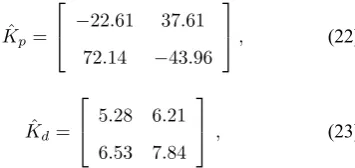
By (18)β=−1/90 =−0.0111. Suppose thath= 0.004, and choose
ˆ
Kp=
⎡
⎣ −22.61 37.61
72.14 −43.96
⎤
⎦, (22)
ˆ
Kd=
⎡
⎣ 5.28 6.21
6.53 7.84
⎤
⎦, (23)
andτ = 0.05. We can compute γ= 0.0099>2h= 0.008, and set α = 0.5γ. The maximum of the real-parts of the closed poles can now be computed as −0.0059, which is less than−h=−0.004. Thus the requirement is fulfilled. In this example,hmax is very small as shown in Fig. 5, due to the fact thatβ is very close to the imaginary-axis.
Example 3.4: The PID-synthesis procedure based on
Proposition 2.1 involves free parameter choices. Consider
the same transfer-function as in (19) of Example 3.1. Let
h = 1, choose τ = 0.05, and set α = 0.5γ as before. If
we choose( ˆKp= 2.5,Kdˆ = 0.2), then the the dash line in Fig. 6 shows the closed-loop step response. However, if we
[image:4.595.362.540.358.442.2]choose( ˆKp= 2,Kdˆ =−0.1), then we obtain a completely different step response as shown with the dash-dotted line in
Fig. 6. It is natural to ask then if the free parameters can be
Consider a prototype second order model plant, withζ= 0.7andωn= 6; i.e.,
Tmodel= ω 2
n s2+ 2ζω+ωn2
(24)
We want the closed-loop step responsesm(t)using the model plant Tmodel to be as close as possible to the actual step response so(t). The step response using Tmodel is shown with the solid line in Fig. 6. Let us consider the cost function
error= 1 3
3
0 (sm(t)−so(t))
2dt, (25)
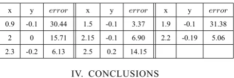
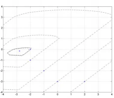
whereso(t)is the step response for any choice of( ˆKp,Kdˆ ). By plotting the contour of the error in terms of( ˆKp,Kdˆ )in Fig. 7, we find the global minimum of the error to occur at
( ˆKp= 1.47,Kdˆ =−0.15). The step response corresponding
to this choice of( ˆKp,Kdˆ )is shown with the solid line with a circle in Fig. 6, which is closer to the model step response
[image:5.595.53.294.417.498.2]than the other two.
Table 2: Evaluated points for contours in Example 3.4
x y error x y error x y error
0.9 -0.1 30.44 1.5 -0.1 3.37 1.9 -0.1 31.38
2 0 15.71 2.15 -0.1 6.90 2.2 -0.19 5.06
2.3 -0.2 6.13 2.5 0.2 14.15
IV. CONCLUSIONS
For stable plants whose poles have negative real-parts less
than a pre-specified−h, we obtained a sufficient condition for existence of PID-controllers that achieve integral-action
and closed-loop poles with real-parts less than−h. We pro-posed a systematic design procedure, which allows freedom
in the choice of parameters. We showed in an example how
this freedom can be used to improve a input
single-output system’s performance. Extending the optimal
parame-ter selection to MIMO systems would be a challenging goal.
These results are limited to stable plants. Future
direc-tions of this study will involve extension to certain classes
of unstable MIMO plants. In addition, optimal parameter
selections for the MIMO case will be explored.
REFERENCES
[1] K. J. Astr¨om and T. Hagglund,PID Controllers: Theory, Design, and Tuning, Second Edition, Research Triangle Park, NC: Instrument Society of America, 1995.
[2] M. Morari, “Robust Stability of Systems with Integral Control,”IEEE Trans. Autom. Control, 47: 6, pp. 574-577, 1985.
[3] M.-T. Ho, A. Datta, S. P. Bhattacharyya, “An extension of the gen-eralized Hermite-Biehler theorem: relaxation of earlier assumptions,” Proc. 1998 American Contr. Conf., pp. 3206-3209, 1998.
[4] G. J. Silva, A. Datta, S. P. Bhattacharyya,PID Controllers for Time-Delay Systems, Birkh¨auser, Boston, 2005.
[5] C.-A. Lin, A. N. G¨undes¸, “Multi-input multi-output PI controller design,”Proc. 39th IEEE Conf. Decision & Control, pp. 3702-3707, 2000.
[6] A. N. G¨undes¸, A. B. ¨Ozg¨uler, “PID stabilization of MIMO plants,” IEEE Transactions on Automatic Control, to appear.
[7] G. C. Goodwin, S. F. Graebe, M. E. Salgado,Control System Design, Prentice Hall, New Jersey, 2001.
[8] M. Vidyasagar,Control System Synthesis: A Factorization Approach, MIT Press, 1985.
[9] K. H. Johansson, “The quadruple-tank process: A multivariable labo-ratory process with an adjustable zero,”IEEE Trans. Control Systems Technology, 8, (3), pp. 456-465, 2000.
- h - C - h? - G
-6
−
r e
v
w y
Fig. 2. Contour ofγ( ˆKp,Kˆd)for Example 3.1
Fig. 3. Findinghmaxfor Example 3.1
[image:6.595.328.522.332.496.2]Fig. 4. Contour ofγ( ˆKp,Kˆd)for Example 3.2
Fig. 5. Findinghmaxfor Example 3.3
Fig. 6. Step responses for Example 3.4
[image:6.595.79.271.333.496.2] [image:6.595.80.270.552.715.2] [image:6.595.328.521.557.718.2]