Dynamic Thresholding Based Edge Detection

Dynamic Thresholding Based Edge Detection

Neeta Nain, Gaurav Jindal, Ashish Garg and Anshul Jain

Abstract—Edges are regions of interest and edge detection is the process of determining where the boundaries of objects fall within an image. It is an important concept, both in the area of object recog-nition and motion tracking. This paper presents an adaptive thresholding based edge-detection method using morphological operators. The novelty of the ap-proach is the adaptive efficient peak detection of the image histogram, thus deciding the modality of image and also the usage of morphological operations in the extraction of one pixel thickm−connected boundary which is continuous in a segment.

Keywords: Peaks,Boundary, Edges, Morphological Op-erations.

1

Introduction

An edge [1], [2], [3], [4] is usually a step change in inten-sity in an image. It corresponds to the boundary between two regions or a set of points in the image where luminous intensity changes very sharply. The presence of an edge within a grayscale image indicates that there is a change in the grayscale from one region to another. The deriva-tive of the grayscale levels within an image as a function of the (x, y) position provides a means of detecting the presence of an edge. A large number of vision applica-tions like matching and tracking use edges and lines as primitives. The process of edge detection is usually fol-lowed(preceded) by the Thresholding of the edge detected image. The process of thresholding provides a means of separating weak edges from strong edges. Consider two adjacent pixels, if these pixels are having dissimilar gray levels, then there is a good probability that they are sepa-rated by gray level discontinuity. This is easier said than done, when dealing with digital pictures, most images are having continuous intensity variation. This leads to edges having a gradual change of pixel levels from one object to the next thus causing the edge to be less defined and harder to distinguish and therefore an optimal threshold value is very important for clearly distinguishing between distinct regions.

The common challenge of good edge detection algorithms is to have a low probability of error i.e; failing to mark edges or falsely marking non-edges with the marked points as close as possible to the center of true edge. Considering the assumption that objects in an image can

∗_{Malaviya National Institute of Technology, Department of}

Computer Engineering, Jaipur, INDIA

be distinguished on the basis of their gray levels, image thresholding technique is being used to determine the var-ious regions into which the image can be segmented. The number of regions into which image can be divided de-pends upon the number of dominant peaks [7] present in the image histogram as explained in section 3.1. After calculating the number of significant peaks, the image is thresholded using Multi-level thresholding technique and than morphological operators(gradient) are used to ex-tract the edges as explained in section 3.3. The edges ob-tained may be more than one pixel thick on the boundary. They are made one-pixel thick by using the various mor-phological thinning masks as explained in subsection 3.4. The extracted boundary is then smoothed to fill one-pixel breaks and to remove erroneous single stray pixels as ex-plained in section 3.5. The proposed method has been evaluated both qualitatively and quantitatively over a number of images with different intensity gradation with excellent results as shown in section 3.5. It identifies all significant edges with minimal false positives.

2

Literature Review

Some of the earliest methods of detecting edges like, Roberts [1], Prewitt [2], Sobel [8] etc in images used small convolution masks to approximate the first derivative of the image brightness function. The most popular gra-dient masks are the Prewitt and Sobel edge detectors. The Sobel edge filter provides good edge detection and is somewhat insensitive to noise present within the im-age. This is due to the averaging that is performed by this edge detector during the computation of the gradi-ent. The most popularly used edge detector is defined by Canny Edge Detector [9]. Since the Canny edge de-tector is a significant and widely used contribution to edge detection techniques and it is also used for our ex-perimental comparisons, its principles are explained in detail. Canny proposed a new approach to edge detec-tion that is optimal for step edges corrupted with white noise. Canny’s derivation of a new edge detector is based on several ideas.

• The edge detector was expressed for a 1D signal. A closed-form solution was found using the calculus of variations.

G is a 2D Gaussian signal and assume we wish to convolve the image with an operator G_n which is the first derivative of Gin the directionn.

G_n= δG

δn =n˙G (1)

The directionnshould be oriented perpendicular to the edge. Iff is the image, the normal to the edge nis estimated as

n= (G∗f)

| (G∗f)| (2) The edge location is then at the local maximum of the image f convolved with the operator G_n in the direction n

δ

δnGn∗f (3)

Substituting in 3 for G_n from equation 1, we get

δ2

δn2G∗f = 0 (4)

The equation 4 illustrates how to find local maxima in the direction perpendicular to the edge; this op-eration is often referred to as non-maximal suppres-sion. The edge strength (magnitude of the gradient of an image intensity function) is measured as

|G_n∗f|=| (G∗f)| (5)

• Noise may cause spurious responses to edge detec-tion, called as ’streaking’ problem. Usually the out-put of the edge detector is thresholded to decide which edges are significant, and streaking means the breaking up of the edge contour caused by the op-erator fluctuating below and above the threshold. Streaking can be removed by thresholding with hys-teresis. If the edge response is above a high thresh-old, those pixels detect definite edges for a particular scale. Individual weak responses usually correspond to noise, but if these pixels are connected to any of the pixels with strong responses, they are more likely to be actual edges in the image. Such connected pix-els are treated as edge pixpix-els if their response is above a low threshold. The low and high thresholds are set according to an estimated signal-to-noise ratio.

3

Image Thresholding

Thresholding [2] is the process of separating an image into different regions based upon its gray level distribu-tion. Key to the selection of a threshold value is an im-age’s histogram, which defines the gray level distribution of its pixels. The bimodal nature of this histogram is typ-ical of images containing two predominant regions of two different gray levels as objects and background. When dealing with digital pictures, most images are having con-tinuous intensity variation and if only a single threshold

level is used then many important regions are lost. It becomes difficult to identify significant regions of such images having multimodal histogram. A better method of Thresholding the gray level image is thus to use mul-tilevel Thresholding [6] instead of bi level thresholding. This is the approach that is taken in the implementa-tion of optimal thresholding. We calculate the optimal number of threshold levels by computing the number of significant peaksfrom image’s histogram as explained below.

3.1

Peak Detection Algorithm

We propose an efficient peak-finding algorithm to deter-mine the number of prodeter-minent peaks in the histogram of the image. The number of peaks [7] represents the num-ber of distinct regions, the image can be divided into. The number of significant peaks are computed as:

1. Compute the frequency histogram of the image. In-sert gray level values and their corresponding fre-quencies into the sets G and F respectively. For each gray leveli, put the element (i,f_i) into the set S0, where f_i is the frequency corresponding to the ithgray level.

S0 ={(i, f_i)} (6) where i G andf_i F.

2. Compute the setS1, that contains the elements rep-resenting the points of local maxima in the image histogram.

S1 ={(i, f_i)|((f_i−1< f_i)&(f_i> f_i+1))} (7) where (i, f_i) S0

3. Compute the set S2 comprising of elements having frequency higher than 1% of the maximum frequency f_max in the set S1. This empirical threshold value 1% is taken as the optimal value based on experi-ments performed over 100sof images having various gradual intensity changes varying from bi level to 9 levels.

f_max=max(F) (8) S2 ={(i, f_i)|f_i> f_max} (9) where (i, f_i) S1

4. Remove the elements having close peaks from setS2. This is done by checking the difference between the gray levels of two elements in setS2. If the difference is less than 20, then the element with lower frequency is removed. Again 20 is an empirically determined threshold value based on experiments. Construct set S3 after the removal of close peaks as:

S3 =S2− {(((i, f_i)|i > j, (i−j)≤20) &(f_i=min(f_i, f_j)))} Proceedings of the World Congress on Engineering 2008 Vol I

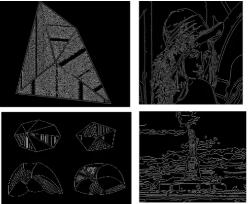
Figure 1: Test images with various gradual variations in intensity a) Object1, image having gradient within the region b)Lena, standard test image with gradual inten-sity change c) Object2, image having gradient within the region and across the regions d) Statue of liberty with light background

where (i, f_i) S2 &j G&f_i, f_j F

5. The number of elements in set S3, denoted as |S3|, is equal to the number of significant peaks in the histogram:

n=|S3| (10)

where nis the number of prominent peaks.

The prominent peaks in image histograms for the images in figure 1 are shown in figure 2.

3.2

Multi-level Thresholding Algorithm

If the input image is a gray level image then the boundary extracted image could be in gray level. To convert the image into a binary image we threshold the image. For thresholding, we compute multilevel thresholds adaptive of local intensity variations as:

1. Compute the frequency histogram of the image. For each gray leveli, the probability distributionp_i =fi

N, where N is the total number of pixels and f_i is the frequency ofith gray level .

2. For M −level thresholding; Divide L, the total number of gray levels, into M classes as C₁[1..t₁], C₂[t₁..t₂], ..., C_M[t_M−1..L] where the total number of thresholds = M −1 and M = n, calculated in equation 10.

Figure 2: a) Image histogram having four prominent peaks, b) Image histogram having six prominent peaks, c) Image histogram having nine prominent peaks, d) Image histogram having five prominent peaks

3. Compute w_k and μ_k for each class k as w_k = iCkpi,μk =

iCk ipi wk 4. Compute the variance σ_B2 as,

σ2_B(t₁, t₂, ..., t_M−1) = M

k=1

(w_kμ2_k−μ2_T) (11)

where μ_T =M_k=1w_kμ_k

5. The optimal thresholds are,

(t∗₁, t∗₂, ..., t∗_M−1) =M ax(σ_B2(t₁, t₂, ..., t_M−1)) (12) where 1≤t₁ < t₂ < ... < t_M−1 < L and σ_B2=M_k=1w_kμ2_k

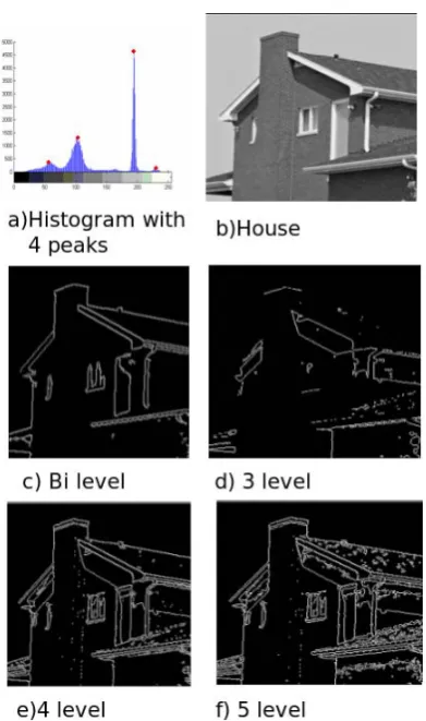
Figure 3: (a) Intensity histogram of original image hav-ing 4 peaks, (b) Original image, (c) Two threshold classes, (d) Three threshold classes, (e) Four threshold classes(optimal), (f) Five threshold classes

and 3-level thresholding in Figures 3(c),(d) does not re-flect the gradual intensity changes within the house and hence the internal details of the house are missed. Fig-ure 3(e) gives good edges when four threshold classes are used(computed using our optimal threshold method). In-creasing the number of thresholds beyond the number of peaks increases the noise in the image as shown in figure 3(f).

3.3

Edge Detection

A powerful set of binary image processing operations de-veloped from a set-theoretical approach comes under the heading of mathematical morphology [2]. Although the basic operations are simple, the operations and their vari-ants can be concatenated to produce much more complex effects. In the general case, morphological image pro-cessing operates by passing astructuring element(StrEl) over the image in an activity similar to convolution. The structuring element can be of any size, and it can contain any complement of 1sand 0s, and a−1 specifies don’t care. At each pixel position a specified logical operation is performed between the structuring element and the

underlying binary image. The binary result of that logi-cal operation is stored in the output image at that pixel position. The effect created depends upon the size and content of the structuring element and upon the nature of the logical operation. All the morphological operators used here conform to their standard definition [2]. The morphological operations of erosion(conforms to gradi-ent) is used to detect edges. The set difference between the original object and the eroded(dilated) object pro-duces a contour that straddles the inside(outside) of the contour of the original object. The inside contour of the thresholded image or the edge detector is defined as:

img=img−(imgStrEl) (13) Where the,

StrEl=

⎡

⎣01 11 01 0 1 0

⎤ ⎦

can be used to erode the image andis morphological erosion operation.

3.4

Boundary Thinning

The result of step 3.3 is a boundary extracted image which can be two or more pixel thick image. To con-vert the above two or more pixel thick edge extracted image to one pixel thick image, we search extra pixels in each direction using Hit-and-Miss transform. The set of 3 x 3 masks;

M ask1 =

⎡

⎣10 11 11 0 −1 0

⎤ ⎦

and M ask2 =

⎡

⎣11 11 10 0 −1 0

⎤ ⎦

will search extra pixels in the horizontal direction. By rotating these masks by 90◦ we get the masks for ver-tical direction and by rotating these masks by 45◦ we can get the masks for diagonal direction too. M ask1 and M ask2 finds extra pixels in positive and negative directions respectively. Using these masks we compute theHit-and-Miss Transformof the image and remove the pixels searched by these masks. This step performs thin-ning(identifies the medial axis) of the boundary and con-verts the two or more pixel thick boundary to one-pixel thick boundary.

3.5

Remove Noisy Stray Pixels and Fill in

Pixel Breaks

The Hit-and-Miss transform may create pixel breaks in the image boundary as shown in Fig 4(a-e) and may Proceedings of the World Congress on Engineering 2008 Vol I

Figure 4: a) Isolated pixel and One pixel break in a straight horizontal or vertical line(one pixel thick), b) One pixel break in a straight horizontal line and there is only one pixel above the break, c) One pixel thick diago-nal line with one extra pixel in 4-neighborhood of any of the pixel of this diagonal, d), e) One pixel thick straight line with one extra pixel above any of the pixels in the line, f) A ”T” made by a set of pixels

also create single stray pixels. For making a continu-ous boundary and to reduce noise, these pixel breaks are to be filled in and the isolated noisy pixels are to be re-moved. ToThin and toFill gaps in the binary image we used the set of masks shown in Figure 5(with rotation of 90◦four times on each masks). The output after applying the above masks to Figure 4(I) is shown in Figure 4(II). A pixelpat coordinates (x, y) has two horizontal and two vertical neighbors whose coordinates are (x+ 1, y),(x− 1, y),(x, y+ 1)and(x, y−1). This set of 4−neighbors of p denoted as N₄(p) are called 4-connected and simi-larly the four diagonal neighbors ofphaving coordinates (x+ 1, y+ 1),(x+ 1, y−1),(x−1, y+ 1)and(x−1, y−1) are denoted as N_D(p). The union of N₄(p) and N_D(p) are the 8−neighborsofpdenoted asN₈(p). If a pixelp

Figure 5: Masks to Thin and Fill in Gaps

Figure 6: Edge extraction results using Proposed Bound-ary extractor on test images shown in Figure 1

is both 4-and 8-connected toqit introduces redundancy in path fromptoq which can be avoided by converting their connectivity to m-connectivity. Two pixels p and q arem-connected whenq ∈ N₄(p) orq ∈ N_D(p) AND N₄(p)N₈(q) = ∅. To obtain m−connected boundary from the above one pixel thick boundary

M ask7 =

⎡

⎣01 11 00 0 0 0

⎤ ⎦

is used for a Hit-miss transform and the pixels searched byM ask7 are subtracted from the boundary as:

bdry=bdry−(bdry⊗M ask7) (14) where⊗is Hit-Miss transform. This step removes redun-dancy in connectivity and the boundary pixels becomes m-connected.

4

Test Results

Figure 7: Edge extraction results using Canny Boundary extractor on test images shown in Figure 1

removed and internal details of statue image are detected using the proposed edge extractor, Figures 6c), 6d). The results obtained using the dynamic Multi level threshold-ing technique show remarkable improvement in contrast to the bi level thresholding used in most of the common edge extractors.

5

Conclusions

This paper proposes a novel and efficient method which uses morphological operations for detection of edges or boundary. All significant edges are identified as Multi-level optimal thresholds are computed. Compared to tra-ditional convolution derivative masks for edge detection morphological operations are used which are efficient, as they are applied on the complete image while convolu-tion masks are applied at every pixel posiconvolu-tion. Compared to existing Edge detectors like Canny [9] and Roberts, Prewitt [2] etc., our algorithm extracts precise one pixel thick seamless, continuous (in a segment) image bound-ary which is very important to extract prominent and significant corners [10] in images and also in computing image semantics [11]. This method works on all types of images, noise suppression is handled by Gaussian smooth-ing withσ= 4.95. This method can further be extended to handle all type of noises like Poisson, Speckle and Gaussian noise withσ >1. Furthermore, while convert-ing boundary sconvert-ingle pixel thick, thinnconvert-ing in all directions is done, which could be alternatively done by local non-maxima suppression perpendicular to the edge direction. This could improve edge localization.

References

[1] V Hlavac M Sonka and R Boyle, Image Processing Analysis and Machine Vision, Chapman and Hall, 1993.

[2] Rafael C. Gonzalez and Richard E. Woods, Digital Image Processing, Addison Wesley Longman, 2nd ed., 2000.

[3] H Itoh J T Law and H Seki, Image Filtering, Edge Detection, and Edge Tracing Using Fuzzy Reasoning. IEEE Transactions on Pattern Analysis and Machine Intelligence, 1996, vol. 18, pp. 481–491.

[4] D Marr and E Hildreth, Theory of Edge Detection. Computer Vision, Los Alamitos, CA, 1991, pp. 77– 107.

[5] N Otsu, A Threshold Selection Method from Gray Level Histograms. IEEE Transactions on Systems Man Cybernet, 1979, vol. SMC-9, pp. 62–66.

[6] Ping-Sung Liao, Tse-Sheng Chen and Pau-Choo Chung A Fast Algorithm for Multi-level Thresholding . Journal of Information Science and Engineering, 2001, vol. 17, pp.713-727.

[7] H Oulhadj A Nakib and P Siarry, Image Histogram Thresholding Based on Multiobjective Optimization. Signal Processing, November,2007, vol. 87, pp. 2516– 2534.

[8] L G Roberts, Machine Perception of Three-Dimensional Solids, Optical and Electro-Optical In-formation Processing, MIT Press, Cambridge, MA, 1965.

[9] J F Canny, A Computational Approach to Edge De-tection. IEEE Transactions on Pattern Analysis and Machine Intelligence, 1986, vol. 8(6), pp. 679–698.

[10] Neeta Nain, Vijay Laxmi, Bhavitavya Bhadviya and Arpita Gopal, Corner Detection Using Difference Chain Code as Curvature. The Third IEEE Interna-tional Conference on Signal Image Technology and Internet Based Systems, SITIS‘07, 2007, vol. Track III, pp. 766–770.

[11] Neeta Nain, Vijay Laxmi, Deepak Agarwal and Man-ish Khandelwal, in Transformation Invariant Shape Descriptors. International Conference on Image Pro-cessing and Computer Vision, IPCV’07, June 25-28, Nevada, USA, 2007, vol. I, pp. 545–550.