Synchronizing Coloring Of A Directed Graph
N. Karimi
∗Abstract—A synchronizing of a deterministic au-tomaton is a word in the alphabet of colors ( consid-ered as letters ) of its edges that maps the automaton to a single state. A coloring of edges of a directed graph is synchronizing if the coloring turns the graph into a deterministic finite automaton possessing a syn-chronizing word.
The road coloring problem is synchronizing coloring of a directed finite strongly connected graph with con-stant out-degree of all its vertices if the greatest com-mon divisor of lengths of all its cycles is one. The problem was posed by Adler, Goodwin and Weiss over 30 years ago and evoked noticeable interest among the specialists in the theory of graphs, deterministic au-tomata and symbolic dynamics.
After so many people challenge to solve this prob-lem finally, A.N Trahtman could present a positive solution. Therefore we know that we can make a syn-chronizing coloring for every graph witch has the nec-essary conditions. In this note we are going to explain a method for appointing a synchronizing coloring and a synchronizing word, in some special cases.
1
Introduction
Let us call a directed graph G = (V, E) admissible (k -admissible to be precise) if all vertices have the same out-degreek. A deterministic finite automaton (D F A) without initial and final states is obtained if we color the edges of a k-admissible directed graph with k colors in such a way that allkedges leaving any node have distinct colors. Let = {1,2, ..., k} be the labeling alphabet. We use the standard notation ∗ for the set of words over . Every word w∈ ∗ defines a state transition functionfw : V → V on the vertex set V. The vertex
fw(v) is the end point of the unique path that starts at
v and whose labels read w. For a set S ⊆V we define
fw(S) = {fw(v)|v ∈S} andfw−1(S) = {v | fw(v) ∈S}. Wordwis called synchronizing iffw(V) is a singleton set and the automaton is called synchronized.
We have presented a method for making a synchronized automaton from a directed graph witch has necessary conditions (aperiodic and strongly connected). Note that from then on we consider just 2-admissible graph.
∗Faculty Member Of Islamic Azad University Farahan Branch,
Email: karimi@Iau-farahan.ac.ir
2
preliminaries
Definition 2.1. Let G= (V, E) be a directed gragh. G
is said to be strongly connected if there should be a path inGbetween any two vertices.
Definition 2.2. LetG= (V, E)be a directed gragh. Gis said to be aperiodic ifV can not be partitioned into sets
V1, V2, . . . , Vd =V0(d > 1) in manner that for all edges
(u, υ)if u∈Vi thenυ∈Vi+1.
It is easy to show that the graph is aperiodic if and only if thegcdof the lengths of its cycles is one.
Definition 2.3. Let G = (V, E) be a 2-admissible di-rected gragh. Let
φ:E(G)−→ {r, b} uυ−→φ(uυ)
as for everyu∈V(G)ifuυ anduυare the only two out edges ofu, then φ(uυ)=φ(uυ). Then we say (G, φ) is a colored graph.
Let (G, φ) be a colored graph. Let = {r, b} be the labeling alphabet. We use the standard notation∗ for the set of words over. Every wordw∈∗ defines a state transition functionfw :V −→V on the vertex set
V; the vertexfw(υ) is the end point of the unique path starting atυ and whose labels readw. For a set S ⊆V
we define fw(S) = {fw(v) | v ∈ S} and fw−1(S) = {v | fw(v)∈S}.
Definition 2.4. Wordwis called synchronizing iffw(V)
is a singleton set, and the automaton is called synchro-nized if a synchronizing word exists. A coloring of an 2-admissible directed graph is synchronized if the corre-sponding automaton is synchronized.
Definition 2.5. If word w is a synchronizing such that
fw(V) ={v} then we callv a final vertex.
Definition 2.6. The matrixA= [aij](n+1)×(n+1)is said
to be an adjacency matrix of the graph G if
aij =
1 υiυj∈E(G) 0 otherwise
where i = 0,1, . . . , n and j = 0,1, . . . , n and V =
{υ0, υ1, . . . , υn}.
rij =
1 aij = 1 φ(vivj) =r 0 o.w.
bij =
1 aij= 1 φ(vivj) =b
0 o.w.
wherei= 0,1, . . . , n and j= 0,1, . . . , n. It is clear that
A=B+R.
The road coloring conjecture: if G is an aperiodic and strongly connected admissible directed gragh, then it has synchronized coloring.
3
Coloring of
G
In this section we have described our method for coloring of G. Before starting to describe our method, it would be better to explain the main idea which leads to this method.
LetGbe a strongly connected and aperiodic 2-admissible directed gragh andV ={vo, v1, . . . , vn}.
Let G have synchronizing word with final vertex v0
and w = w1w2. . .wf. So, fw(v0) = v0, fw(v1) =
v0, . . . , fw(vn) =v0.
Definition 3.1. Let T ⊆ V. Assume that the sets of in-edges and in-neighbors ofT are denoted as follows:
E(T) ={e∈E(G)|e=uv; u∈V, v∈T}, I(T) ={u∈V(G) | ∃v∈T; uv∈E(G)}.
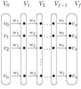
LetT0={v0},Tk =I(Tk−1) fork= 1,2, . . . , f. And let
[image:2.595.97.226.594.736.2]S0=E(T0),Sk−1=E(Tk−1) fork= 1,2, . . . , f.
Figure 1 shows all the paths between everyvi to v0
fol-lowingw’s letters.
V0 V1 V2 Vf−1 Vf
v0−→ •w1 −→ •w2 . . .•−→ •vwf o
v1−→ •w1 −→ •w2 . . .•−→ •wf vo v2−→ •w1 −→ •w2 . . .•−→ •wf vo
.. .
vn−→ •w1 −→ •w2 . . .•−→ •vwf o
Figure 1. Wordwwith final vertexv0.
LetV0=V andVk=fwk(Vk−1) fork= 1,2, . . . , f, and
let Ek = {e = uv ∈ E(G)|u ∈ Vk−1, φ(e) = wk} for
k= 1,2, . . . , f.
It is clear that Vk ⊆ Tf−k and Ek ⊆ Sf−k for k = 1, . . . , f.
On the other hand, all edges inEk have the same color. Thus if we try to color G, in such a way that Sf−k to become mono-color as mush as possible, then, we can reach a synchronizing coloring.
How to color a graph:
Let arbitrary vertexv0 be the final vertex. (Since G is strongly connected, the existence of synchronizing word is independent of the choice ofν0.)
Point 3.1. If v0 is a vertex which has maximum in-degree, then the length ofw will be shorter.
Then, not ignoring generality, we color all of members
S0 with one of “Red” or “Blue” colors arbitrary, if any
e= (uv)∈S0is colored withr(b) we will colore = (uv) withb(r). (Every vertex has 2 out degree.)
Then, we continue to color members of S1 that haven’t been colored yet. Since, at first we consider to color the edges in S1. If blue edges are more than red edges in
S1, we will color the remaining edges inS1with blue and otherwise with red (as a greedy way).
Point 3.2. If there are2 edges in Si for i≥1 which is leaving one common vertex, then we must not color them with a same color.
Then, we continue to colorS2, . . . , Sk, . . . in this way as far as all of edges are colored. In fact, we colorGin such a way that all of non-colored edges betweenTk+1 andTk become mono-colored (as a greedy way relying point 3.1).
Decomposing of A to R and B:
Now we try to decompose matrixA(adjacency matrix of
G) to coloring matricesRandBaccording to the coloring method described at the beginning of the section. We will define matrixA from the matrixA such thatA= [aij]
aij =
Z aij = 0
0 aij = 0 Z =r, b, then we will findRandB according toA.
LetKbe theKth column of matrixA, that has maximum number of 1’s, if all columns have the same number of 1’s, we can choose any column. We change all 1’s in the columnK by “r”.
We will illustrate each satge by our example of matrixA,
A= ⎡ ⎢ ⎢ ⎢ ⎢ ⎣
0 1 0 0 1
0 1 1 0 0
1 0 0 1 0
1 0 0 0 1
0 0 1 1 0
⎤ ⎥ ⎥ ⎥ ⎥ ⎦.
We takeK = 1 and color 1’s in column byr, then color next 1’s in rows 3 and 4 byb.
A= ⎡ ⎢ ⎢ ⎢ ⎢ ⎣
0 1 0 0 1
0 1 1 0 0
r 0 0 b 0
r 0 0 0 b
0 0 1 1 0
⎤ ⎥ ⎥ ⎥ ⎥ ⎦
Figure 2. Coloring of rows 3 and 4 of matrixA.
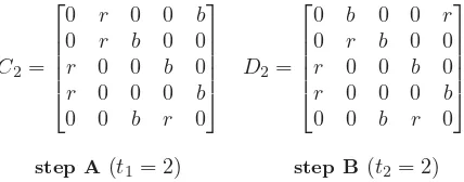
Then we consider the rows ofAwhich have been colored in the previous stage (rows 3, 4 in fig. 2) and continue to color the columns of the same number (columns 3, 4 in fig. 2). Firstly, we will check two below steps. In this step if there is no 1 in matrix A we will stop coloring. Otherwise, there will be at least a non colored 1 in these columns, becauseGis strongly connected.
step A: We start to change all of remained 1’s with r
as much as possible. (Note that when we change every 1 entry in a row we must change the other 1 in that row with opposite color at once.) Then lett1be the difference between the number ofr’s andb’s in these columns.
step B: We start to change all of remained 1’s withbas much as possible. Then lett2 be the difference between the number ofr’s andb’s in these columns.
(In figure 3 we have colored matrixAin figure 2 according steps A and B.)
C1= ⎡ ⎢ ⎢ ⎢ ⎢ ⎣
0 1 0 0 1
0 b r 0 0
r 0 0 b 0
r 0 0 0 b
0 0 r b 0
⎤ ⎥ ⎥ ⎥ ⎥ ⎦ D1=
⎡ ⎢ ⎢ ⎢ ⎢ ⎣
0 1 0 0 1
0 r b 0 0
r 0 0 b 0
r 0 0 0 b
0 0 b r 0
⎤ ⎥ ⎥ ⎥ ⎥ ⎦
[image:3.595.312.526.116.200.2]step A(t1= 0) step B (t2= 2)
Figure 3. We color columns 3 and 4 in fig. 2 accordoing steps A and B and lett1 andt2be the difference between the numbers ofrs andb’s in these columns respectively.
Now if t1 < t2, then we continue coloring with step B. Otherwise, we continue with step A.
If there exists any 1 in matrixAwe continue coloring by this process, frist we consider non zero rows of previous colored columns (rows 2, 3, 5 of columns 3, 4 in figure 3), then we colore the new columns which their numbers are the same as the numbers of the deretmined rows in frist step (columns 2, 3, 5). we color these new columns based on steps A and B. (See figure 4.)
C2= ⎡ ⎢ ⎢ ⎢ ⎢ ⎣
0 r 0 0 b
0 r b 0 0
r 0 0 b 0
r 0 0 0 b
0 0 b r 0
⎤ ⎥ ⎥ ⎥ ⎥ ⎦ D2=
⎡ ⎢ ⎢ ⎢ ⎢ ⎣
0 b 0 0 r
0 r b 0 0
r 0 0 b 0
r 0 0 0 b
0 0 b r 0
⎤ ⎥ ⎥ ⎥ ⎥ ⎦
step A(t1= 2) step B (t2= 2)
Figure 4. Coloring ofA=D1according steps A and B.
If there is no 1 in matrixAwe are in the final stage and we stop. But if in the final staget1=t2we select coloring matrixA as follows: Let
rDf = number of columns includingrin matrixDf,
bDf = number of columns includingb in matrixDf,
rCf = number of columns includingrin matrixCf,
bCf = number of columns includingb in matrixCf, andm= min{rDf, rCf, bDf, bCf}.
Ifm=rC or m=bC thenA =Cf, otherwiseA=Df. Then we will get matrixR andB based onA.
In our example we see thatrD2 =bD2 = 4,rC2 =bC2= 3
andm= min{rD2, rC2, bD2, bC2}=rD2 =rC2.
There-foreA =C2. (See figure 5.)
R= ⎡ ⎢ ⎢ ⎢ ⎢ ⎣
0 r 0 0 0
0 r 0 0 0
r 0 0 0 0
r 0 0 0 0
0 0 0 r 0
⎤ ⎥ ⎥ ⎥ ⎥
⎦ B =
⎡ ⎢ ⎢ ⎢ ⎢ ⎣
0 0 0 0 b
0 0 b 0 0
0 0 0 b 0
0 0 0 0 b
0 0 b 0 0
⎤ ⎥ ⎥ ⎥ ⎥ ⎦
[image:3.595.312.524.470.557.2]A =C2=R+B
Figure 5. Decomposing of coloring matrixAto two coloring matricesRandB.
4
Constructing synchronizing word
We construct synchronizing word as follows: Let
V0 = {v0, v1, . . . , vn} = V; we define subsets V1, V2, . . .
fromV0, inductively.
Vrk:=φr(Vk−1) Vb
k =φb(Vk−1)
Vb
k=Sbk Vrk=Srk
Vk := ⎧ ⎨ ⎩
Vrk Srk ≤Sb
k, Vrk =Vrj, Vrk=Vbj
(j= 1,2, . . . , k−1)
[image:3.595.53.272.535.616.2]If there exist somef ∈N such that:
|Vrf|= 1 or|Vb f|= 1,
and
|Vri| = 1 and|Vb
i| = 1 for alli < f,
thenw=w1w2. . . wf, where
wk=
r Vk=Vrk b Vk=Vbk wis the synchronizing word.
If we want to describe our method based on matrix product, indeed, we want to find a sequence ofR’s and
B’s matrices such that products of them is a matrix that has one column with all entries 1. Ifw is synchronizing word then the matrixW =W1W2. . .Wf in which
Wi:=
[rij] wi=r
[bij] wi=b (i= 1,2, . . . , f),
and by replacingr’s andb’s with 1. This is easy to show thatW has just one column with all entries 1.
We have constructed an algorithm based on this way to find synchronizing word and have written its program by Q basic language. We have verified many various exam-ples with our algorithm . We have written this program based on the matrix productsR’s orB’s matrices. There are examples in which our algorithms are not finishing. In other word, for everyk= 1,2, . . .|Vrk| = 1 and|Vbk| = 1. So, we will have two cases in hand:
A: We will run into a loop of a proper subset ofV.
B: We will run into a loop of all vertices ofV.
We guess that in case A,Gis not strongly connected and that in case B,Gis periodic.
5
Examples
In the following examplesAis an adjacency matrix. We presented our examples in different shapes, but all shapes are based on our method:
Example 1:A= ⎡ ⎢ ⎢ ⎢ ⎢ ⎣
0 1 0 0 1
0 1 1 0 0
1 0 0 1 0
1 0 0 0 1
0 0 1 1 0
⎤ ⎥ ⎥ ⎥ ⎥ ⎦
Figure [2, 3, 4, 5]=⇒
R= ⎡ ⎢ ⎢ ⎢ ⎢ ⎣
0 r 0 0 0
0 r 0 0 0
r 0 0 0 0
r 0 0 0 0
0 0 0 r 0
⎤ ⎥ ⎥ ⎥ ⎥
⎦ B =
⎡ ⎢ ⎢ ⎢ ⎢ ⎣
0 0 0 0 b
0 0 b 0 0
0 0 0 b 0
0 0 0 0 b
0 0 b 0 0
⎤ ⎥ ⎥ ⎥ ⎥ ⎦ ↓
v0 v1 v2 v3 v4 v1 v1 v0 v0 v3
v0 v1 v3 v1 v1 v0
v0 v1 v1 v1
=⇒ Synchronizing word is: “rrr”. Note that there are some other words such as “brb”.
Example 2 : A =
⎡ ⎢ ⎢ ⎢ ⎢ ⎣
0 0 1 0 1
0 1 0 1 0
1 0 0 0 1
0 1 1 0 0
0 1 0 1 0
⎤ ⎥ ⎥ ⎥ ⎥
⎦ Starts from the
second column, R= ⎡ ⎢ ⎢ ⎢ ⎢ ⎣
0 0 0 0 r
0 r 0 0 0
0 0 0 0 r
0 r 0 0 0
0 r 0 0 0
⎤ ⎥ ⎥ ⎥ ⎥
⎦ B=
⎡ ⎢ ⎢ ⎢ ⎢ ⎣
0 0 b 0 0
0 0 0 b 0
b 0 0 0 0
0 0 b 0 0
0 0 0 b 0
⎤ ⎥ ⎥ ⎥ ⎥ ⎦
step 1: φr({v0, v1, v2, v3, v4}) ={v1, v4}=C1
φb({v0, v1, v2, v3, v4}) ={v0, v2, v3}=D1
step 2: φr(C1) ={v1} φb(C1) ={v3}
=⇒Synchronizing words are: “rr” with final vertex: v1, and “rb” with final vertex: v3.
Example 3 : A =
⎡ ⎢ ⎢ ⎢ ⎢ ⎣
0 1 0 1 0
0 0 1 0 1
1 0 0 1 0
1 0 1 0 0
0 0 1 0 1
⎤ ⎥ ⎥ ⎥ ⎥
⎦ Starts from the
third column R= ⎡ ⎢ ⎢ ⎢ ⎢ ⎣
0 0 0 r 0
0 0 r 0 0
r 0 0 0 0
0 0 r 0 0
0 0 r 0 0
⎤ ⎥ ⎥ ⎥ ⎥
⎦ B =
⎡ ⎢ ⎢ ⎢ ⎢ ⎣
0 b 0 0 0
0 0 0 0 b
0 0 0 b 0
b 0 0 0 0
0 0 0 0 b
⎤ ⎥ ⎥ ⎥ ⎥ ⎦ ↓
v0 v1 v2 v3 v4 v3 v2 v0 v2 v2
v0 v2 v3 v1 v3 v0
v0 v1 v3 v3 v2 v2
v2 v3 v0 v2
v0 v2 v3 v0
v0 v3 v1 v0
v0 v1 v1 v4
v1 v4 v2 v2
[image:4.595.295.541.211.424.2]
Eample 4:A= ⎡ ⎢ ⎢ ⎣
0 1 0 1
1 0 1 0
0 1 0 1
1 0 1 0
⎤ ⎥ ⎥ ⎦
R= ⎡ ⎢ ⎢ ⎣
0 r 0 0
r 0 0 0
0 r 0 0
r 0 0 0 ⎤ ⎥ ⎥
⎦ B =
⎡ ⎢ ⎢ ⎣
0 0 0 b
0 0 b 0
0 0 0 b
0 0 b 0
⎤ ⎥ ⎥ ⎦
↓
v0 v1 v2 v3 v1 v0 v1 v0
v0 v1 v3 v2
v2 v3 v1 v0
=⇒ We run into a loop of all vertices of V; and G is periodic.
Acknowledgement
We express our warm thanks with Professor B. Nash-vadiyan for his helps to us in editing.
References
[1] R. L. Adler, L.W. Goodwyn, and B. Weiss., Equiv-alence of topological Markov shifts, Israel j. Math. 27 : 49−63,(1977).
[2] G.L. O’Brien., The road-coloring problem, Israel j. Math. 39 : 145−154,(1981)
[3] J. Friedman., On the road coloring, Proc. Amer. Math. Soc. 110 : 1133−1135,(1990).
[4] J. Kari.,Synchronizing finite automata on Eulerian digragh, Theoret. comput. sci, 295(1−3) : 223− 232,(2003).
[5] R.L. Adler and B. Weiss., Similarity of
automor-phisms of the torus, Memooirs of the American
mathemathical society, providence, RI, 1970.
![Figure [2, 3, 4, 5]=⎢⎢⎢⎢⎣⇒](https://thumb-us.123doks.com/thumbv2/123dok_us/1308149.660818/4.595.295.541.211.424/figure.webp)
