Cutting off Redundant Repeating Generations for Neural Abstractive Summarization

Cutting-off Redundant Repeating Generations

for Neural Abstractive Summarization

Jun Suzuki and Masaaki Nagata

NTT Communication Science Laboratories, NTT Corporation 2-4 Hikaridai, Seika-cho, Soraku-gun, Kyoto, 619-0237 Japan

{suzuki.jun, nagata.masaaki}@lab.ntt.co.jp

Abstract

This paper tackles the reduction of re-dundant repeating generation that is often observed in RNN-based encoder-decoder models. Our basic idea is to jointly esti-mate the upper-bound frequency of each target vocabulary in the encoder and con-trol the output words based on the estima-tion in the decoder. Our method shows significant improvement over a strong RNN-based encoder-decoder baseline and achieved its best results on an abstractive summarization benchmark.

1 Introduction

The RNN-based encoder-decoder (EncDec) ap-proach has recently been providing signifi-cant progress in various natural language gen-eration (NLG) tasks, i.e., machine translation (MT) (Sutskever et al., 2014; Cho et al., 2014) and abstractive summarization (ABS) (Rush et al., 2015). Since a scheme in this approach can be interpreted as a conditional language model, it is suitable for NLG tasks. However, one potential weakness is that it sometimes repeatedly generates the same phrase (or word).

This issue has been discussed in the neural MT (NMT) literature as a part of a coverage prob-lem (Tu et al., 2016; Mi et al., 2016). Such re-peating generation behavior can become more se-vere in some NLG tasks than in MT. The very shortABS task in DUC-2003 and 2004 (Over et al., 2007) is a typical example because it requires the generation of a summary in a pre-defined lim-ited output space, such as ten words or 75 bytes. Thus, the repeated output consumes precious lim-ited output space. Unfortunately, the coverage ap-proach cannot be directly applied to ABS tasks since they require us to optimally find salient ideas

from the input in alossy compressionmanner, and thus the summary (output) length hardly depends on the input length; an MT task is mainlyloss-less generation and nearly one-to-one correspondence between input and output (Nallapati et al., 2016a). From this background, this paper tackles this is-sue and proposes a method to overcome it in ABS tasks. The basic idea of our method is to jointly estimate the upper-bound frequency of each tar-get vocabulary that can occur in a summary during the encoding process and exploit the estimation to control the output words in each decoding step. We refer to our additional component as a word-frequency estimation (WFE) sub-model. The WFE sub-model explicitly manages how many times each word has been generated so far and might be generated in the future during the decod-ing process. Thus, we expect to decisively prohibit excessive generation. Finally, we evaluate the ef-fectiveness of our method on well-studied ABS benchmark data provided by Rush et al. (2015), and evaluated in (Chopra et al., 2016; Nallapati et al., 2016b; Kikuchi et al., 2016; Takase et al., 2016; Ayana et al., 2016; Gulcehre et al., 2016).

2 Baseline RNN-based EncDec Model

The baseline of our proposal is an RNN-based EncDec model with an attention mechanism (Lu-ong et al., 2015). In fact, this model has al-ready been used as a strong baseline for ABS tasks (Chopra et al., 2016; Kikuchi et al., 2016) as well as in the NMT literature. More specifically, as a case study we employ a2-layer bidirectional LSTMencoder and a2-layer LSTMdecoder with a global attention (Bahdanau et al., 2014). We omit a detailed review of the descriptions due to space limitations. The following are the necessary parts for explaining our proposed method.

Let X = (xi)Ii=1 and Y = (yj)Jj=1 be input and output sequences, respectively, wherexi and

Input:Hs= (hs_i)I_i=1 .list of hidden states generated by encoder Initialize:s←0 .s: cumulative log-likelihood

ˆ

Y ←‘BOS0 .Yˆ: list of generated words

Ht←Hs .Ht_{: hidden states to process decoder} 1: h←(s,Yˆ,Ht) .triplet of (minimal) info for decoding process

2: Qw←push(Qw, h) .set initial triplethto priority queueQw

3: Qc← {} .prepare queue to store complete sentences 4: Repeat

5: O˜←() .prepare empty list

6: Repeat

7: h←pop(Qw) .pop a candidate history

8: o˜←calcLL(h) .see Eq. 2

9: O˜←append( ˜O,o˜) .append likelihood vector

10: UntilQw=∅ .repeat untilQwis empty

11: {( ˆm,ˆk)z}K−C

z=1 ←findKBest( ˜O) 12: {hz}K−C

z=1 ←makeTriplet({( ˆm,ˆk)z}K−Cz=1 ) 13: Q0_{←selectTopK(Q}

c,{hz}K−Cz=1 )

14: (Qw,Qc)←SepComp(Q0) .separateQ0intoQcorQw

15: UntilQw=∅ .finish ifQwis empty

Output:Qc

Figure 1: Algorithm for aK-best beam search de-coding typically used in EncDec approach.

yj are one-hot vectors, which correspond to the

i-th word in the input and thej-th word in the out-put. Let Vt _{denote the vocabulary (set of words)} of output. For simplification, this paper uses the following four notation rules:

(1) (xi)I_i=1 is a short notation for representing a list of (column) vectors, i.e., (x1, . . . ,xI) =

(xi)Ii=1.

(2)v(a, D)represents aD-dimensional (column) vector whose elements are all a, i.e., v(1,3) = (1,1,1)>_.

(3)x[i]represents thei-th element ofx,i.e.,x= (0.1,0.2,0.3)>_{, thenx[2] = 0.2.}

(4)M=|Vt_{|and,malways denotes the index of} output vocabulary, namely,m ∈ {1, . . . , M}, and

o[m]represents the score of them-th word inVt_, whereo∈RM_.

Encoder: LetΩs_{(·)denote the overall process} of our 2-layer bidirectional LSTM encoder. The encoder receives inputX and returns a list of final hidden statesHs_{= (h}s

i)Ii=1:

Hs_{= Ω}s_{(X). (1)}

Decoder: We employ aK-best beam-search de-coder to find the (approximated) best output Yˆ

given input X. Figure 1 shows a typical K -best beam search algorithm used in the decoder of EncDec approach. We define the (minimal) re-quired informationhshown in Figure 1 for thej -th decoding process is -the following triplet, h = (sj−1,Yˆj−1,Hjt−1), where sj−1 is the cumula-tive log-likelihood from step 0 to j − 1, Yˆj−1

is a (candidate of) output word sequence gener-ated so far from step 0 toj−1, that is,Yˆj−1 =

(y0, . . . ,yj−1) and H_jt₋₁ is the all the hidden states for calculating the j-th decoding process. Then, the functioncalcLLin Line 8 can be writ-ten as follows:

˜

oj =v sj−1, M+ log Softmax(oj)

oj = Ωt Hs,Hjt−1,yˆj−1, (2)

where Softmax(·) is the softmax function for a given vector andΩt_{(·)represents the overall} pro-cess of a single decoding step.

Moreover, O˜ in Line 11 is a (M×(K−C)) -matrix, whereC is the number of complete sen-tences in Qc. The (m, k)-element of O˜

repre-sents a likelihood of them-th word, namelyo˜j[m], that is calculated using the k-th candidate in Qw

at the (j −1)-th step. In Line 12, the function

makeTripletconstructs a set of triplets based on the information of index( ˆm,ˆk). Then, in Line 13, the functionselectTopKselects the top-K

candidates from union of a set of generated triplets at current step {hz}K_z=1−Cand a set of triplets of complete sentences in Qc. Finally, the function

sepCompin Line 13 divides a set of tripletsQ0_in

two distinct sets whether they are complete sen-tences, Qc, or not, Qw. If the elements in Q0

are all complete sentences, namely,Qc = Q0 and Qw =∅, then the algorithm stops according to the

evaluation of Line 15.

3 Word Frequency Estimation

This section describes our proposed method, which roughly consists of two parts: (1) a sub-model that estimates the upper-bound frequencies of the target vocabulary words in the output, and (2) architecture for controlling the output words in the decoder using estimations.

3.1 Definition

Let aˆ denote a vector representation of the fre-quency estimation.denotes element-wise prod-uct.aˆ is calculated by:

ˆ

a= ˆrgˆ ˆ

r=ReLU(r), gˆ=Sigmoid(g), (3)

where Sigmoid(·) and ReLu(·) represent the element-wise sigmoid and ReLU (Glorot et al., 2011), respectively. Thus, rˆ ∈ [0,+∞]M_{, gˆ ∈}

We incorporate two separated components, rˆ

andgˆ, to improve the frequency fitting. The pur-pose ofgˆis to distinguish whether the target words occur or not, regardless of their frequency. Thus,

ˆ

g can be interpreted as a gate function that re-sembles estimating the fertility in the coverage (Tu et al., 2016) and a switch probability in the copy mechanism (Gulcehre et al., 2016). These ideas originated from such gated recurrent networks as LSTM (Hochreiter and Schmidhuber, 1997) and GRU (Chung et al., 2014). Then,rˆcan much fo-cus on to model frequency equal to or larger than 1. This separation can be expected sincer[ˆm]has no influence ifg[ˆm]=0.

3.2 Effective usage

The technical challenge of our method is effec-tively leveraging WFEaˆ. Among several possible choices, we selected to integrate it as prior knowl-edge in the decoder. To do so, we re-defineo˜j in Eq. 2 as:

˜

oj =v sj−1, M+ log (Softmax(oj)) + ˜aj. The difference is the additional term ofa˜j, which is an adjusted likelihood for the j-th step origi-nally calculated fromaˆ. We definea˜jas:

˜

aj = log (ClipReLU1(˜rj)g)ˆ . (4)

ClipReLU₁(·) is a function that receives a

vec-tor and performs an element-wise calculation:

x0_{[m] = max (0,min(1,x[m])) for allm if it}

re-ceives x. We define the relation between r˜j in Eq. 4 andrˆin Eq. 3 as follows:

˜ rj =

ˆ

r ifj= 1

˜

rj−1−yˆj−1 otherwise . (5) Eq. 5 is updated fromr˜j−1tor˜jwith the estimated output of previous stepyˆj−1. Sinceyˆj∈ {0,1}M for all j, all of the elements in r˜j are monoton-ically non-increasing. If r˜j0[m] ≤ 0 at j0, then

˜

oj0[m]=−∞regardless ofo[m]. This means that

them-th word will never be selected any more at step j0 _{≤ j for all j. Thus, the interpretation of}

˜

rjis that it directly manages the upper-bound fre-quency of each target word that can occur in the current and future decoding time steps. As a result, decoding with our method never generates words that exceed the estimation rˆ, and thus we expect to reduce the redundant repeating generation.

Note here that our method never requires

˜

rj[m]≤0(orr˜j[m] = 0) for allmat the last de-coding time stepj, as is generally required in the

Input:Hs= (hs_i)I_i=1 .list of hidden states generated by encoder Parameters: W₁r,W₁g∈RH×H,W₂r∈RM×H, W₂g∈

RM×2H_,

1: H₁r←W₁rHs .linear transformation for frequency model

2: hr₁←H₁rv(1, M) .hr

1∈RH,H1r∈RH×I 3: r←W₂rhr₁ .frequency estimation

4: H₁g ←W₁gHs .linear transformation for occurrence model

5: hg₂+←RowMax(H₁g) .hg+

2 ∈RH, andH1g∈RH×I 6: hg−₂ ←RowMin(H₁g) .hg−

2 ∈RH, andH1g∈RH×I 7: g←W₂g concat(h₂g+,hg−₂ ) _.

occurrence estimation Output:(g,r)

Figure 2: Procedure for calculating the compo-nents of our WFE sub-model.

coverage (Tu et al., 2016; Mi et al., 2016; Wu et al., 2016). This is why we sayupper-bound fre-quency estimation, not just(exact) frequency. 3.3 Calculation

Figure 2 shows the detailed procedure for calcu-latinggandrin Eq. 3. Forr, we sum up all of the features of the input given by the encoder (Line 2) and estimate the frequency. In contrast, forg, we expect Lines 5 and 6 to work as a kind ofvoting for both positive and negative directions since g

needs justoccurrenceinformation, notfrequency. For example, g may take large positive or nega-tive values if a certain input word (feature) has a strong influence for occurring or not occurring specific target word(s) in the output. This idea is borrowed from the Max-pooling layer (Goodfel-low et al., 2013).

3.4 Parameter estimation (Training)

Given the training data, let a∗ _{∈ P}M _{be a} vector representation of the true frequency of the target words given the input, where P =

{0,1, . . . ,+∞}. Clearly a∗ _{can be obtained by}

counting the words in the corresponding output. We define loss function Ψwfe _{for estimating our} WFE sub-model as follows:

Ψwfe _X,a∗_{,W=d·v(1, M) (6)}

d=c1max v(0, M),aˆ−a∗−v(, M)b

+c2max v(0, M),a∗−aˆ−v(, M)b,

whereW represents the overall parameters. The form of Ψwfe_{(·) is closely related to that used} in support vector regression (SVR) (Smola and Sch¨olkopf, 2004). We allow estimationa[ˆ m]for all m to take a value in the range of [a∗_{[m] −} ,a∗_{[m] +]with no penalty (the loss is zero). In}

Source vocabulary †119,507

Target vocabulary †68,887

Dim. of embeddingD 200

Dim. of hidden stateH 400

Encoder RNN unit 2-layer bi-LSTM

Decoder RNN unit 2-layer LSTM with attention Optimizer Adam (first 5 epoch)

+ SGD (remaining epoch)? Initial learning rate 0.001 (Adam) / 0.01 (SGD) Mini batch size 256 (shuffled at each epoch) Gradient clipping 10 (Adam) / 5 (SGD)

Stopping criterion max 15 epoch w/ early stopping based on the val. set

Other opt. options Dropout = 0.3

Table 1: Model and optimization configurations in our experiments. †: including special BOS, EOS, and UNK symbols. ?: as suggested in (Wu et al., 2016)

ofa∗_{are an integer. The remaining 0.25 for both}

the positive and negative sides denotes themargin between every integer. We select b = 2 to pe-nalize larger for more distant error, and c1 < c2, i.e., c1 = 0.2, c2 = 1, since we aim to obtain upper-bound estimation and to penalize the under-estimation below the true frequencya∗_.

Finally, we minimize Eq. 6 with a standard neg-ative log-likelihood objective function to estimate the baseline EncDec model.

4 Experiments

We investigated the effectiveness of our method on ABS experiments, which were first performed by Rush et al., (2015). The data consist of ap-proximately 3.8 million training, 400,000 valida-tion and 400,000 test data, respectively2_.

Gener-ally, 1951 test data, randomly extracted from the test data section, are used for evaluation3_.

Addi-tionally, DUC-2004 evaluation data (Over et al., 2007)4_{were also evaluated by the identical models}

trained on the above Gigaword data. We strictly followed the instructions of the evaluation setting used in previous studies for a fair comparison. Ta-ble 1 summarizes the model configuration and the parameter estimation setting in our experiments.

4.1 Main results: comparison with baseline Table 2 shows the results of the baseline EncDec and our proposed EncDec+WFE. Note that the

2_{The data can be created by the data construction scripts}

in the author’s code: https://github.com/facebook/NAMAS.

3_{As previously described (Chopra et al., 2016) we}

re-moved the ill-formed (empty) data for Gigaword.

4_{http://duc.nist.gov/duc2004/tasks.html}

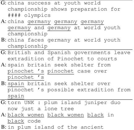
G:china success at youth world championship shows preparation for #### olympics

A:china germany germany germany germany and germany at world youth championship

B:china faces germany at world youth championship

G:British and Spanish governments leave extradition of Pinochet to courts A:spain britain seek shelter from

pinochet ’s pinochet case over pinochet ’s

B:spain britain seek shelter over pinochet ’s possible extradition from spain

G:torn UNK : plum island juniper duo now just a lone tree

A:black women black women black in black code

B:in plum island of the ancient

Figure 3: Examples of generated summary. G: reference summary, A: baseline EncDec, and B: EncDec+WFE. (underlines indicate repeating phrases and words)

DUC-2004 data was evaluated by recall-based ROUGE scores, while the Gigaword data was evaluated by F-score-based ROUGE, respec-tively. For a validity confirmation of our EncDec baseline, we also performed OpenNMT tool5_.

The results on Gigaword data with B = 5

were, 33.65, 16.12, and 31.37 for ROUGE-1(F), ROUGE-2(F) and ROUGE-L(F), respec-tively, which were almost similar results (but slightly lower) with our implementation. This sup-ports that our baseline worked well as a strong baseline. Clearly, EncDec+WFE significantly out-performed the strong EncDec baseline by a wide margin on the ROUGE scores. Thus, we conclude that the WFE sub-model has a positive impact to gain the ABS performance since performance gains were derived only by the effect of incorpo-rating our WFE sub-model.

4.2 Comparison to current top systems Table 3 lists the current top system results. Our method EncDec+WFE successfully achieved the current best scores on most evaluations. This re-sult also supports the effectiveness of incorporat-ing our WFE sub-model.

MRT (Ayana et al., 2016) previously provided the best results. Note that its model structure is nearly identical to our baseline. On the contrary, MRT trained a model with a sequence-wise

DUC-2004 (w/ 75-byte limit) Gigaword (w/o length limit) Method Beam ROUGE-1(R) ROUGE-2(R) ROUGE-L(R) ROUGE-1(F) ROUGE-2(F) ROUGE-L(F)

EncDec B=1 29.23 8.71 25.27 33.99 16.06 31.63

(baseline) B=5 29.52 9.45 25.80 †34.27 †16.68 †32.14

our impl.) B=10 †29.60 †9.62 †25.97 34.18 16.51 31.97

EncDec+WFE B=1 31.92 9.36 27.22 36.21 16.87 33.55

(proposed) B=5 ?32.28 ?10.54 ?27.80 ?36.30 ?17.31 ?33.88

B=10 31.70 10.34 27.48 36.08 17.23 33.73

(perf. gain from†to?) +2.68 +0.92 +1.83 +2.03 +0.63 +1.78 Table 2: Results on DUC-2004 and Gigaword data: ROUGE-x(R): recall-based ROUGE-x,

ROUGE-x(F): F1-based ROUGE-x, wherex∈ {1,2, L}, respectively.

DUC-2004 (w/ 75-byte limit) Gigaword (w/o length limit) Method ROUGE-1(R) ROUGE-2(R) ROUGE-L(R) ROUGE-1(F) ROUGE-2(F) ROUGE-L(F)

ABS (Rush et al., 2015) 26.55 7.06 22.05 30.88 12.22 27.77

RAS (Chopra et al., 2016) 28.97 8.26 24.06 33.78 15.97 31.15

BWL (Nallapati et al., 2016a)1 _{28.35 9.46 24.59 32.67 15.59 30.64}

(words-lvt5k-1sent†) 28.61 9.42 25.24 35.30 †16.64 32.62

MRT (Ayana et al., 2016) †30.41 †10.87 †26.79 †36.54 16.59 †33.44

EncDec+WFE[This Paper] 32.28 10.54 27.80 36.30 17.31 33.88

(perf. gain from†) +1.87 -0.33 +1.01 -0.24 +0.72 +0.44

Table 3: Results of current top systems: ‘*’: previous best score for each evaluation. †: using a larger vocab for both encoder and decoder, not strictly fair configuration with other results.

Truea∗\Estimationaˆ 0 1 2 3 4≥

1 7,014 7,064 1,784 16 4

2 51 95 60 0 0

3≥ 2 4 1 0 0

Table 4: Confusion matrix of WFE on Gigaword data: only evaluated true frequency≥1.

imum risk estimation, while we trained all the models in our experiments with standard (point-wise) log-likelihood maximization. MRT essen-tially complements our method. We expect to fur-ther improve its performance by applying MRT for its training since recent progress of NMT has suggested leveraging a sequence-wise optimiza-tion technique for improving performance (Wise-man and Rush, 2016; Shen et al., 2016). We leave this as our future work.

4.3 Generation examples

Figure 3 shows actual generation examples. Based on our motivation, we specifically selected the re-dundant repeating output that occurred in the base-line EncDec. It is clear that EncDec+WFE suc-cessfully reduced them. This observation offers further evidence of the effectiveness of our method in quality.

4.4 Performance of the WFE sub-model To evaluate the WFE sub-model alone, Table 4 shows the confusion matrix of the frequency

esti-mation. We quantizedaˆbyba[ˆ m]+0.5cfor allm, where 0.5 was derived from the margin in Ψwfe_. Unfortunately, the result looks not so well. There seems to exist an enough room to improve the esti-mation. However, we emphasize that it already has an enough power to improve the overall quality as shown in Table 2 and Figure 3. We can expect to further gain the overall performance by improving the performance of the WFE sub-model.

5 Conclusion

This paper discussed the behavior of redundant repeating generation often observed in neural EncDec approaches. We proposed a method for reducing such redundancy by incorporating a sub-model that directly estimates and manages the fre-quency of each target vocabulary in the output. Experiments on ABS benchmark data showed the effectiveness of our method, EncDec+WFE, for both improving automatic evaluation performance and reducing the actual redundancy. Our method is suitable forlossy compressiontasks such as im-age caption generation tasks.

Acknowledgement

References

Ayana, Shiqi Shen, Zhiyuan Liu, and Maosong Sun. 2016. Neural headline generation with minimum risk training. CoRR, abs/1604.01904.

Dzmitry Bahdanau, Kyunghyun Cho, and Yoshua Ben-gio. 2014. Neural Machine Translation by Jointly Learning to Align and Translate. InProceedings of the 3rd International Conference on Learning Rep-resentations (ICLR 2015).

Kyunghyun Cho, Bart van Merrienboer, Caglar Gul-cehre, Dzmitry Bahdanau, Fethi Bougares, Hol-ger Schwenk, and Yoshua Bengio. 2014. Learn-ing Phrase Representations usLearn-ing RNN Encoder– Decoder for Statistical Machine Translation. In

Proceedings of the 2014 Conference on Empirical Methods in Natural Language Processing (EMNLP 2014), pages 1724–1734.

Sumit Chopra, Michael Auli, and Alexander M. Rush. 2016. Abstractive Sentence Summarization with At-tentive Recurrent Neural Networks. In Proceed-ings of the 2016 Conference of the North Ameri-can Chapter of the Association for Computational Linguistics: Human Language Technologies, pages 93–98, San Diego, California, June. Association for Computational Linguistics.

Junyoung Chung, C¸aglar G¨ulc¸ehre, KyungHyun Cho, and Yoshua Bengio. 2014. Empirical Evaluation of Gated Recurrent Neural Networks on Sequence Modeling. CoRR, abs/1412.3555.

Xavier Glorot, Antoine Bordes, and Yoshua Bengio. 2011. Deep Sparse Rectifier Neural Networks. In Geoffrey J. Gordon and David B. Dunson, ed-itors, Proceedings of the Fourteenth International Conference on Artificial Intelligence and Statistics (AISTATS-11), volume 15, pages 315–323. Journal of Machine Learning Research - Workshop and Con-ference Proceedings.

Ian J. Goodfellow, David Warde-Farley, Mehdi Mirza, Aaron C. Courville, and Yoshua Bengio. 2013. Maxout Networks. In Proceedings of the 30th In-ternational Conference on Machine Learning, ICML 2013, Atlanta, GA, USA, 16-21 June 2013, pages 1319–1327.

Caglar Gulcehre, Sungjin Ahn, Ramesh Nallapati, Bowen Zhou, and Yoshua Bengio. 2016. Point-ing the Unknown Words. In Proceedings of the 54th Annual Meeting of the Association for Compu-tational Linguistics (Volume 1: Long Papers), pages 140–149, Berlin, Germany, August. Association for Computational Linguistics.

Sepp Hochreiter and J¨urgen Schmidhuber. 1997. Long Short-Term Memory. Neural Comput., 9(8):1735– 1780, November.

Yuta Kikuchi, Graham Neubig, Ryohei Sasano, Hi-roya Takamura, and Manabu Okumura. 2016. Con-trolling output length in neural encoder-decoders.

In Proceedings of the 2016 Conference on Empiri-cal Methods in Natural Language Processing, pages 1328–1338, Austin, Texas, November. Association for Computational Linguistics.

Thang Luong, Hieu Pham, and Christopher D. Man-ning. 2015. Effective Approaches to Attention-based Neural Machine Translation. In Proceed-ings of the 2015 Conference on Empirical Methods in Natural Language Processing, pages 1412–1421, Lisbon, Portugal, September. Association for Com-putational Linguistics.

Haitao Mi, Baskaran Sankaran, Zhiguo Wang, and Abe Ittycheriah. 2016. Coverage embedding models for neural machine translation. In Proceedings of the 2016 Conference on Empirical Methods in Nat-ural Language Processing, pages 955–960, Austin, Texas, November. Association for Computational Linguistics.

Ramesh Nallapati, Bing Xiang, and Bowen Zhou. 2016a. Sequence-to-sequence rnns for text summa-rization. CoRR, abs/1602.06023.

Ramesh Nallapati, Bowen Zhou, Cicero dos Santos, Caglar Gulcehre, and Bing Xiang. 2016b. Ab-stractive Text Summarization using Sequence-to-sequence RNNs and Beyond. InProceedings of The 20th SIGNLL Conference on Computational Natural Language Learning, pages 280–290, Berlin, Ger-many, August. Association for Computational Lin-guistics.

Paul Over, Hoa Dang, and Donna Harman. 2007. DUC in context. Information Processing and Manage-ment, 43(6):1506–1520.

Alexander M. Rush, Sumit Chopra, and Jason We-ston. 2015. A Neural Attention Model for Abstrac-tive Sentence Summarization. InProceedings of the 2015 Conference on Empirical Methods in Natural Language Processing (EMNLP 2015), pages 379– 389.

Shiqi Shen, Yong Cheng, Zhongjun He, Wei He, Hua Wu, Maosong Sun, and Yang Liu. 2016. Mini-mum risk training for neural machine translation. In

Proceedings of the 54th Annual Meeting of the As-sociation for Computational Linguistics (Volume 1: Long Papers), pages 1683–1692, Berlin, Germany, August. Association for Computational Linguistics. Alex J Smola and Bernhard Sch¨olkopf. 2004. A tu-torial on support vector regression. Statistics and computing, 14(3):199–222.

Ilya Sutskever, Oriol Vinyals, and Quoc V. Le. 2014. Sequence to Sequence Learning with Neural Net-works. InAdvances in Neural Information Process-ing Systems 27 (NIPS 2014), pages 3104–3112. Sho Takase, Jun Suzuki, Naoaki Okazaki, Tsutomu

In Proceedings of the 2016 Conference on Empiri-cal Methods in Natural Language Processing, pages 1054–1059, Austin, Texas, November. Association for Computational Linguistics.

Zhaopeng Tu, Zhengdong Lu, Yang Liu, Xiaohua Liu, and Hang Li. 2016. Modeling Coverage for Neural Machine Translation. InProceedings of the 54th An-nual Meeting of the Association for Computational Linguistics (Volume 1: Long Papers), pages 76–85, Berlin, Germany, August. Association for Computa-tional Linguistics.

Sam Wiseman and Alexander M. Rush. 2016.

Sequence-to-sequence learning as beam-search opti-mization. InProceedings of the 2016 Conference on Empirical Methods in Natural Language Process-ing, pages 1296–1306, Austin, Texas, November. Association for Computational Linguistics.