Latent Tree Language Model
Tom´aˇs Brychc´ın
NTIS – New Technologies for the Information Society, Faculty of Applied Sciences, University of West Bohemia,
Technick´a 8, 306 14 Plzeˇn, Czech Republic
[email protected] nlp.kiv.zcu.cz
Abstract
In this paper we introduce Latent Tree Lan-guage Model (LTLM), a novel approach to language modeling that encodes syntax and semantics of a given sentence as a tree of word roles.
The learning phase iteratively updates the trees by moving nodes according to Gibbs sampling. We introduce two algorithms to in-fer a tree for a given sentence. The first one is based on Gibbs sampling. It is fast, but does not guarantee to find the most probable tree. The second one is based on dynamic program-ming. It is slower, but guarantees to find the most probable tree. We provide comparison of both algorithms.
We combine LTLM with 4-gram Modified Kneser-Ney language model via linear inter-polation. Our experiments with English and Czech corpora show significant perplexity re-ductions (up to 46% for English and 49% for Czech) compared with standalone 4-gram Modified Kneser-Ney language model.
1 Introduction
Language modeling is one of the core disciplines in natural language processing (NLP). Automatic speech recognition, machine translation, optical character recognition, and other tasks strongly de-pend on the language model (LM). An improve-ment in language modeling often leads to better performance of the whole task. The goal of lan-guage modeling is to determine the joint probabil-ity of a sentence. Currently, the dominant approach is n-gram language modeling, which decomposes
the joint probability into the product of conditional probabilities by using thechain rule. In traditional n-gram LMs the words are represented as distinct symbols. This leads to an enormous number of word combinations.
In the last years many researchers have tried to capture words contextual meaning and incorporate it into the LMs. Word sequences that have never been seen before receive high probability when they are made of words that are semantically similar to words forming sentences seen in training data. This ability can increase the LM performance because it reduces thedata sparsity problem. In NLP a very common paradigm for word meaning representation is the use of the Distributional hypothesis. It sug-gests that two words are expected to be semanti-cally similar if they occur in similar contexts (they are similarly distributed in the text) (Harris, 1954). Models based on this assumption are denoted as dis-tributional semantic models (DSMs).
Recently, semantically motivated LMs have be-gun to surpass the ordinary n-gram LMs. The most commonly used architectures are neural network LMs (Bengio et al., 2003; Mikolov et al., 2010; Mikolov et al., 2011) andclass-based LMs. Class-based LMs are more related to this work thus we investigate them deeper.
Brown et al. (1992) introduced class-based LMs of English. Their unsupervised algorithm searches classes consisting of words that are most probable in the given context (one word window in both di-rections). However, the computational complex-ity of this algorithm is very high. This approach was later extended by (Martin et al., 1998;
taker and Woodland, 2003) to improve the complex-ity and to work with wider context. Deschacht et al. (2012) used the same idea and introduced La-tent Words Language Model (LWLM), where word classes are latent variables in a graphical model. They apply Gibbs sampling or the expectation max-imization algorithm to discover the word classes that are most probable in the context of surround-ing word classes. A similar approach was pre-sented in (Brychc´ın and Konop´ık, 2014; Brychc´ın and Konop´ık, 2015), where the word clusters de-rived from various semantic spaces were used to im-prove LMs.
In above mentioned approaches, the meaning of a word is inferred from the surrounding words inde-pendently of their relation. An alternative approach is to derive contexts based on the syntactic relations the word participates in. Such syntactic contexts are automatically produced by dependency parse-trees. Resulting word representations are usually less top-ical and exhibit more functional similarity (they are more syntactically oriented) as shown in (Pad´o and Lapata, 2007; Levy and Goldberg, 2014).
Dependency-based methods for syntactic parsing have become increasingly popular in NLP in the last years (K¨ubler et al., 2009). Popel and Mareˇcek (2010) showed that these methods are promising direction of improving LMs. Recently, unsuper-vised algorithms for dependency parsing appeared in (Headden III et al., 2009; Cohen et al., 2009; Spitkovsky et al., 2010; Spitkovsky et al., 2011; Mareˇcek and Straka, 2013) offering new possibili-ties even for poorly-resourced languages.
In this work we introduce a new DSM that uses tree-based context to create word roles. The word role contains the words that are similarly distributed over similar tree-based contexts. The word role encodes the semantic and syntactic properties of a word. We do not rely on parse trees as a prior knowl-edge, but we jointly learn the tree structures and word roles. Our model is a soft clustering, i.e. one word may be present in several roles. Thus it is the-oretically able to capture the word polysemy. The learned structure is used as a LM, where each word role is conditioned on its parent role. We present the unsupervised algorithm that discovers the tree struc-tures only from the distribution of words in a training corpus (i.e. no labeled data or external sources of
in-formation are needed). In our work we were inspired by class-based LMs (Deschacht et al., 2012), unsu-pervised dependency parsing (Mareˇcek and Straka, 2013), and tree-based DSMs (Levy and Goldberg, 2014).
This paper is organized as follows. We start with the definition of our model (Section 2). The pro-cess of learning the hidden sentence structures is ex-plained in Section 3. We introduce two algorithms for searching the most probable tree for a given sen-tence (Section 4). The experimental results on En-glish and Czech corpora are presented in Section 6. We conclude in Section 7 and offer some directions for future work.
2 Latent Tree Language Model
In this section we describe Latent Tree Language Model (LTLM). LTLM is a generative statistical model that discovers the tree structures hidden in the text corpus.
LetLbe a word vocabulary with total of|L| dis-tinct words. Assume we have a training corpus w
divided into S sentences. The goal of LTLM or other LMs is to estimate the probability of a text P(w). Let Ns denote the number of words in the
s-th sentence. The s-th sentence is a sequence of wordsws = {ws,i}Ni=0s , wherews,i ∈ L is a word
at position iin this sentence and ws,0 = <s>is
an artificial symbol that is added at the beginning of each sentence.
Each sentencesis associated with the dependency graph Gs. We define the dependency graph as a
labeled directed graph, where nodes correspond to the words in the sentence and there is a label for each node that we callrole. Formally, it is a triple
Gs= (Vs,Es,rs)consisting of:
• The set of nodes Vs = {0,1, ..., Ns}. Each
tokenws,iis associated with nodei∈Vs.
• The set of edgesEs⊆Vs×Vs.
• The sequence of rolesrs = {rs,i}Ni=0s , where
1≤rs,i≤K fori∈Vs. K is the number of
roles.
The artificial wordws,0 =<s>at the beginning
of the sentence has always role 1 (rs,0 = 1).
Anal-ogously tow, the sequence of allrsis denoted asr
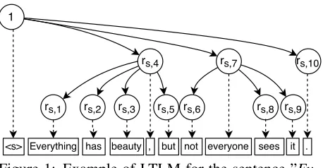
Figure 1: Example of LTLM for the sentence ” Ev-erything has beauty, but not everyone sees it.”
Edge e ∈ Es is an ordered pair of nodes (i, j).
We say thatiis thehead or theparent andjis the dependent or thechild. We use the notationi → j for such edge. The directed path from nodeito node jis denoted asi→∗ j.
We place a few constraints on the graphGs.
• The graphGsis atree. It means it is the acyclic
graph (ifi → j then notj →∗ i), where each node has one parent (ifi → j then notk → j for everyk6=i).
• The graphGs isprojective(there are no cross
edges). For each edge(i, j)and for eachk be-tweeniandj(i.e. i < k < j ori > k > j) there must exist the directed pathi→∗ k.
• The graphGsis always rooted in the node 0.
We denote these graphs as theprojective depen-dency trees. Example of such a tree is on Figure 1. For the treeGswe define a function
hs(j) =i, when(i, j)∈Es (1)
that returns the parent for each node except the root. We use graph Gs as a representation of the
Bayesian network with random variables Es and
rs. The rolesrs,i represent the node labels and the
edges express the dependences between the roles. The conditional probability of the role at position igiven its parent role is denoted asP(rs,i|rs,hs(i)).
The conditional probability of the word at position i in the sentence given its role rs,i is denoted as
P(ws,i|rs,i).
We model the distribution over words in the sen-tencesas the mixture
P(ws) =P(ws|rs,0) =
Ns
Y
i=1
K
X
k=1
P(ws,i|rs,i=k)P(rs,i=k|rs,hs(i)). (2)
The root role is kept fixed for each sentence (rs,0
= 1) soP(ws) =P(ws|rs,0).
We look at the roles as mixtures over child roles and simultaneously as mixtures over words. We can represent dependency between roles with a set ofK multinomial distributionsθ overK roles, such that P(rs,i|rs,hs(i) = k) = θ
(k)
rs,i. Simultaneously,
de-pendency of words on their roles can be represented as a set ofK multinomial distributionsφover |L| words, such thatP(ws,i|rs,i=k) =φ(wks,i) . To make
predictions about new sentences, we need to assume a prior distribution on the parametersθ(k)andφ(k).
We place a Dirichlet prior D with the vector of K hyper-parameters α on a multinomial
distribu-tionθ(k) ∼D(α)and with the vector of|L| hyper-parametersβon a multinomial distributionφ(k) ∼ D(β). In general,Dis not restricted to be Dirichlet distribution. It could be any distribution over dis-crete children, such as logistic normal. In this paper, we focus only on Dirichlet as a conjugate prior to the multinomial distribution and derive the learning algorithm under this assumption.
The choice of the child role depends only on its parent role, i.e. child roles with the same parent are mutually independent. This property is especially important for the learning algorithm (Section 3) and also for searching the most probable trees (Section 4). We do not place any assumption on the length of the sentenceNsor on how many children the parent
node is expected to have.
3 Parameter Estimation
In this section we present the learning algorithm for LTLM. The goal is to estimate θ and φ in a way
that maximizes the predictive ability of the model (generates the corpus with maximal joint probability P(w)).
Letχk(i,j)be an operation that changes the treeGs
toG0s
such that the newly created tree G0(V0s,E0s,r0s) consists of:
• V0s=Vs.
• E0s= (Es\ {(hs(i), i)})∪ {(j, i)}.
• rs,a0 =
rs,a fora6=i
k fora=i, where0≤a≤Ns. It means that we change the role of the selected node i so that rs,i = k and simultaneously we
change the parent of this node to bej. We call this operation apartial change.
The newly created graphG0 must satisfy all con-ditions presented in Section 2, i.e. it is a projec-tive dependency tree rooted in the node 0. Thus not all partial changesχk
(i,j) are possible to perform on
graphGs.
Clearly, for the sentence s there is at most
Ns(1+Ns)
2 parent changes1.
To estimate the parameters of LTLM we apply Gibbs sampling and gradually sampleχk(i,j)for trees
Gs. For doing so we need to determine the posterior
predictive distribution2
G0s∼P(χk(i,j)(Gs)|w,G), (4)
from which we will sample partial changes to update the trees. In the equation,Gdenote the sequence of
all trees for given sentenceswandG0sis a result of
one sampling. In the following text we derive this equation under assumptions from Section 2.
The posterior predictive distribution of Dirichlet multinomial has the form of additive smoothing that is well known in the context of language modeling. The hyper-parameters of Dirichlet prior determine how much is the predictive distribution smoothed. Thus the predictive distribution for the word-in-role distribution can be expressed as
P(ws,i|rs,i,w\s,i,r\s,i) =
n(ws,i|rs,i)
\s,i +β
n(•|rs,i)
\s,i +|L|β
, (5)
1The most parent changes are possible for the special case
of the tree, where each nodeihas parenti−1. Thus for each nodeiwe can change its parent to any nodej < iand keep the projectivity of the tree. That isNs(1+Ns)
2 possibilities.
2The posterior predictive distribution is the distribution of
an unobserved variable conditioned by the observed data, i.e. P(Xn+1|X1, ..., Xn), where Xi are i.i.d. (independent and
identically distributed random variables).
where n(ws,i|rs,i)
\s,i is the number of times the role
rs,i has been assigned to the word ws,i,
exclud-ing the position i in the s-th sentence. The sym-bol•represents any word in the vocabulary so that n(•|rs,i)
\s,i =
P
l∈Ln
(l|rs,i)
\s,i . We use the symmetric
Dirichlet distribution for the word-in-role probabili-ties as it could be difficult to estimate the vector of hyper-parameters β for large word vocabulary. In
the above mentioned equation,βis a scalar.
The predictive distribution for the role-by-role distribution is
P rs,i|rs,hs(i),r\s,i
= n
(rs,i|rs,hs(i)) \s,i +αrs,i
n(•|rs,hs(i)) \s,i +
K
P
k=1
αk
. (6)
Analogously to the previous equation, n(rs,i|rs,hs(i))
\s,i denote the number of times the
role rs,i has the parent role rs,hs(i), excluding the
position i in the s-th sentence. The symbol • represents any possible role to make the probability distribution summing up to 1. We assume an asymmetric Dirichlet distribution.
We can use predictive distributions of above men-tioned Dirichlet multinomials to express the joint probability that the role at positioniisk(rs,i = k)
with parent at positionjconditioned on current val-ues of all variables, except those in positioniin the sentences
P(rs,i=k, j|w,r\s,i)∝
P(ws,i|rs,i=k,w\s,i,r\s,i)
× P(rs,i=k|rs,j,r\s,i)
× Q
a:hs(a)=i
P(rs,a|rs,i=k,r\s,i).
(7)
The choice of the node irole affects the word that is produced by this role and also all the child roles of the nodei. Simultaneously, the role of the node idepends on its parentjrole. Formula 7 is derived from the joint probability of a sentencesand a tree
Gs, where all probabilities which do not depend on
the choice of the role at positioniare removed and equality is replaced by proportionality (∝).
P(χk(i,j)(Gs)|w,G)∝
P(rs,i=k, j|w,r\s,i)
P(rs,i, hs(i)|w,r\s,i)
(8) that is essentially the fraction between the joint probability of rs,i and its parent after the partial
change and before the partial change (conditioned on all other variables). This fraction can be in-terpreted as the necessity to perform this partial change.
We investigate two strategies of sampling partial changes:
• Per sentence: We sample a single partial change according to Equation 8 for each sen-tence in the training corpus. It means during one pass through the corpus (one iteration) we performSpartial changes.
• Per position: We sample a partial change for each position in each sentence. We perform in totalN =PSs=1Nspartial changes during one
pass. Note that the denominator in Equation 8 is constant for this strategy and can be removed. We compare both training strategies in Section 6. After enough training iterations, we can estimate the conditional probabilities φ(lk) and θk(p) from actual samples as
φ(lk)≈ n
(ws,i=l|rs,i=k)+β
n(•|rs,i=k)+|L|β (9)
θk(p) ≈ n
(rs,i=k|rs,hs(i)=p)+α
k
n(•|rs,hs(i)=p)+
K
P
m=1
αm
. (10)
These equations are similar to equations 5 and 6, but here the counts ndo not exclude any position in a corpus.
Note that in the Gibbs sampling equation, we assume that the Dirichlet parameters α and β are given. We use a fixed point iteration technique de-scribed in (Minka, 2003) to estimate them.
4 Inference
In this section we present two approaches for search-ing the most probable tree for a given sentence as-suming we have already estimated the parametersθ
andφ.
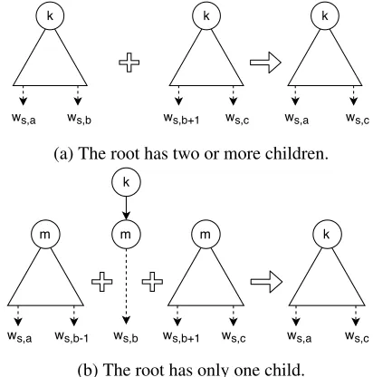
(a) The root has two or more children.
[image:5.612.321.527.57.265.2](b) The root has only one child.
Figure 2: Searching the most probable subtrees.
4.1 Non-deterministic Inference
We use the same sampling technique as for estimat-ing parameters (Equation 8), i.e. we iteratively sam-ple the partial changesχk(i,j). However, we use equa-tions 9 and 10 for predictive distribuequa-tions of Dirich-let multinomials instead of 5 and 6. In fact, these equations correspond to the predictive distributions over the newly added wordws,iwith the rolers,iinto
the corpus, conditioned onwandr. This sampling
technique rarely finds the best solution, but often it is very near.
4.2 Deterministic Inference
Here we present the deterministic algorithm that guarantees to find the most probable tree for a given sentence. We were inspired by Cocke-Younger-Kasami (CYK) algorithm (Lange and Leiß, 2009).
Let Tns,a,c denote the subtree of Gs (subgraph
of Gs that is also a tree) containing subsequence
of nodes {a, a+ 1, ..., c}. The superscript n de-notes the number of children the root of this tree has. We denote the joint probability of a sub-tree from position a to position c with the cor-responding words conditioned by the root role k as Pn({ws,i}ic=a,Tns,a,c|k). Our goal is to find
the tree Gs = T1+s,0,Ns that maximizes probability
P(ws,Gs) =P1+({ws,i}Ni=0s ,T1+s,0,Ns|0).
fol-lows bottom-up direction and goes through all pos-sible subsequences for a sentence (sequence of words). At the beginning, the probabilities for sub-sequences of length 1 (i.e. single words) are calcu-lated asP1+({w
s,a},T1+s,a,a|k) =P(ws,a|rs,a=k).
Once it has considered subsequences of length 1, it goes on to subsequences of length 2, and so on.
Thanks to mutual independence of roles under the same parent, we can find the most probable subtree with the root rolekand with at least two root chil-dren according to
P2+({ws,i}ic=a,T2+s,a,c|k) = max b:a<b<c
[P1+({ws,i}bi=a,T1+s,a,b|k)×
P1+({ws,i}ci=b+1,T1+s,b+1,c|k)]. (11)
It means we merge two neighboring subtrees with the same root rolek. This is the reason why the new subtree has at least two root children. This formula is visualized on Figure 2a. Unfortunately, this does not cover all subtree cases. We find the most proba-ble tree with only root child as follows
P1({ws,i}ci=a,T1s,a,c|k) = max b,m:a≤b≤c,1≤m≤K
[P(ws,b|rs,b=m)×P(rs,b=m|k)×
P1+({ws,i}ib=−a1,T1+s,a,b−1|m)×
P1+({ws,i}ci=b+1,T1+s,b+1,c|m)]. (12)
This formula is visualized on Figure 2b.
To find the most probable subtree no matter how many children the root has, we need to take the maximum from both mentioned equations P1+ =
max(P2+, P1).
The algorithm has complexity O(Ns3K2), i.e. it has cubic dependence on the length of the sentence Ns.
5 Side-dependent LTLM
Until now, we presented LTLM in its simplified ver-sion. In role-by-role probabilities (role conditioned on its parent role) we did not distinguish whether the role is on the left side or the right side of the parent. However, this position keeps important information about the syntax of words (and their roles).
We assume separate multinomial distributions θ˙
for roles that are on the left andθ¨for roles on the
right. Each of them has its own Dirichlet prior with hyper-parameters α˙ andα¨, respectively. The
pro-cess of estimating LTLM parameters is almost the same. The only difference is that we need to rede-fine the predictive distribution for the role-by-role distribution (Equation 6) to include only counts of roles on the appropriate side. Also, every time the role-by-role probability is used we need to distin-guish sides:
P(rs,i|rs,hs(i)) =
( ˙ θ(rs,hs(i))
rs,i fori < hs(i))
¨ θ(rs,hs(i))
rs,i fori > hs(i))
.
(13) In the following text we always assume the side-dependent LTLM.
6 Experimental Results and Discussion
In this section we present experiments with LTLM on two languages, English (EN) and Czech (CS).
As a training corpus we use CzEng 1.0 (Bojar et al., 2012) of the sentence-parallel Czech-English corpus. We choose this corpus because it contains multiple domains, it is of reasonable length, and it is parallel so we can easily provide comparison be-tween both languages. The corpus is divided into 100 similarly-sized sections. We use parts 0–97 for training, the part 98 as a development set, and the last part 99 for testing.
We have removed all sentences longer than 30 words. The reason was that the complexity of the learning phase and the process of searching most probable trees depends on the length of sentences. It has led to removing approximately a quarter of all sentences. The corpus is available in a tokenized form so the only preprocessing step we use is lower-casing. We keep the vocabulary of 100,000 most fre-quent words in the corpus for both languages. The less frequent words were replaced by the symbol <unk>. Statistics for the final corpora are shown in Table 1.
Corpora Sentences Tokens OOV rate
[image:7.612.317.542.53.203.2] [image:7.612.74.301.57.144.2]EN train 11,530,604 138,034,779 1.30% EN develop. 117,735 1,407,210 1.28% EN test 117,360 1,405,106 1.33% CS train 11,832,388 133,022,572 3.98% CS develop. 120,754 1,353,015 4.00% CS test 120,573 1,357,717 4.03% Table 1: Corpora statistics. OOV ratedenotes the out-of-vocabulary rate.
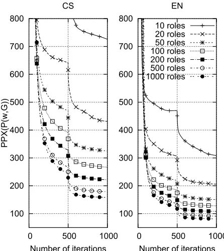
Figure 3: Learning curves of LTLM for both English and Czech. The points in the graphs represent the perplexities in every 100th iteration.
During the process of parameter estimation we measure the perplexity of joint probability of sen-tences and their trees defined asPPX(P(w,G)) =
N
q 1
P(w,G), whereN is the number of all words in
the training dataw.
As we describe in Section 3, there are two ap-proaches for the parameter estimation of LTLM. During our experiments, we found that the per-position strategy of training has the ability to con-verge faster, but to a worse solution compared to the per-sentence strategy which converges slower, but to a better solution.
We train LTLM by 500 iterations of the per-position sampling followed by another 500 iterations of the per-sentence sampling. This proves to be
effi-Model EN CS
2-gram MKN 165.9 272.0
3-gram MKN 67.7 99.3
4-gram MKN 46.2 73.5
300n RNNLM 51.2 69.4
4-gram LWLM 52.7 81.5
PoS STLM 455.7 747.3
1000r STLM 113.7 211.0
1000r det. LTLM 54.2 111.1
4-gram MKN + 300n RNNLM 36.8 (-20.4%) 49.5 (-32.7%) 4-gram MKN + 4-gram LWLM 41.5 (-10.2%) 62.4 (-15.1%)
4-gram MKN + PoS STLM 42.9 (-7.1%) 63.3 (-13.9%)
4-gram MKN + 1000r STLM 33.6 (-27.3%) 50.1 (-31.8%)
4-gram MKN + 1000r det. LTLM 24.9 (-43.1%) 37.2 (-49.4%)
Table 2: Perplexity results on the test data. The numbers in brackets are the relative improvements compared with standalone 4-gram MKN LM.
cient in both aspects, the reasonable speed of con-vergence and the satisfactory predictive ability of the model. The learning curves are showed on Fig-ure 3. We present the models with 10, 20, 50, 100, 200, 500, and 1000 roles. The higher role cardinal-ity models were not possible to create because of the very high computational requirements. Similarly to the training of LTLM, the non-deterministic in-ference uses 100 iterations of per-position sampling followed by 100 iterations of per-sentence sampling. In the following experiments we measure how well LTLM generalizes the learned patterns, i.e. how well it works on the previously unseen data. Again, we measure the perplexity, but of prob-ability P(w) for mutual comparison with differ-ent LMs that are based on differdiffer-ent architectures (PPX(P(w)) = Nq 1
P(w)).
To show the strengths of LTLM we compare it with several state-of-the-art LMs. We experi-ment with Modified Kneser-Ney (MKN) interpola-tion (Chen and Goodman, 1998), with Recurrent Neural Network LM (RNNLM) (Mikolov et al., 2010; Mikolov et al., 2011)3, and with LWLM
(De-schacht et al., 2012)4. We have also created
syntac-tic dependency tree based LM (denoted as STLM). Syntactic dependency trees for both languages are provided within CzEng corpus and are based on
3Implementation is available athttp://rnnlm.org/.
Size of the hidden layer was set to 300 in our experiments. It was computationally intractable to use more neurons.
4Implementation is available at http://liir.cs.
[image:7.612.71.294.184.434.2]EN CS
[image:8.612.75.539.57.147.2]Model\roles 10 20 50 100 200 500 1000 10 20 50 100 200 500 1000 STLM 408.5 335.2 261.7 212.6 178.9 137.8 113.7 992.7 764.2 556.4 451.0 365.9 265.7 211.0 non-det. LTLM 329.5 215.1 160.4 126.5 105.6 86.7 78.4 851.0 536.6 367.4 292.6 235.2 186.1 157.6 det. LTLM 252.4 166.4 115.3 92.0 75.4 60.9 54.2 708.5 390.2 267.8 213.2 167.9 133.5 111.1 4-gram MKN + STLM 42.7 41.6 39.9 37.9 36.3 34.9 33.6 67.5 65.1 61.4 58.3 55.5 52.4 50.1 4-gram MKN + non-det. LTLM 41.1 38.0 35.2 32.7 30.7 28.9 27.8 65.8 59.4 55.1 51.1 47.5 43.7 41.3 4-gram MKN + det. LTLM 39.9 36.4 32.8 30.3 28.1 26.0 24.9 64.4 56.1 51.5 47.3 43.4 39.9 37.2
Table 3: Perplexity results on the test data for LTLMs and STLMs with different number of roles. Deter-ministic inference is denoted asdet. and non-deterministic inference asnon-det.
MST parser (McDonald et al., 2005). We use the same architecture as for LTLM and experiment with two approaches to represent the roles. Firstly, the roles are given by the part-of-speech tag (denoted as PoS STLM). No training is required, all information come from CzEng corpus. Secondly, we learn the roles using the same algorithm as for LTLM. The only difference is that the trees are kept unchanged. Note that both deterministic and non-deterministic inference perform almost the same in this model so we do not distinguish between them.
We combine baseline 4-gram MKN model with other models via linear combination (in the tables denoted by the symbol+) that is simple but very ef-ficient technique to combine LMs. Final probability is then expressed as
P(w) =
S
Y
s=1
Ns
Y
i=1
λPLM1+ (λ−1)PLM2. (14)
In the case of MKN the probability PMKN is the probability of a wordws,iconditioned by 3 previous
words with MKN smoothing. For LTLM or STLM this probability is defined as
PLTLM(ws,i|rs,hs(i)) =
K
X
k=1
P(ws,i|rs,i=k)P(rs,i=k|rs,hs(i)). (15)
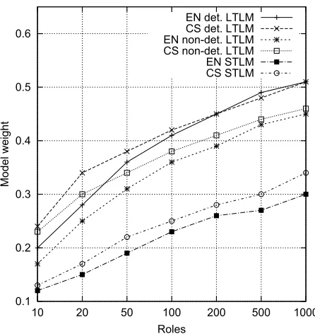
We use the expectation maximization algorithm (Dempster et al., 1977) for the maximum likelihood estimate ofλparameter on the development part of the corpus. The influence of the number of roles on the perplexity is shown in Table 3 and the final
0.1 0.2 0.3 0.4 0.5 0.6
10 20 50 100 200 500 1000
Model weight
Roles
EN det. LTLM CS det. LTLM EN non-det. LTLM CS non-det. LTLM EN STLM CS STLM
Figure 4: Model weights optimized on development data when interpolated with 4-gram MKN LM.
results are shown in Table 2. Note that these per-plexities are not comparable with those on Figure 3 (PPX(P(w))vs. PPX(P(w,G))). Weights of
LTLM and STLM when interpolated with MKN LM are shown on Figure 4.
[image:8.612.314.537.197.433.2]signifi-everything has beauty , but not everyone sees it .
it ’s one , but was he saw him .
that is thing ; course it i made it !
let was life – though not she found her ...
there knows name - or this they took them ’
something really father ... perhaps that that gave his what
nothing says mother : and the it told me “
everything comes way maybe now who felt a how
here does wife ( although had you thought out why
someone gets place ? yet <unk> someone knew that –
god has idea naught except all which heard himself
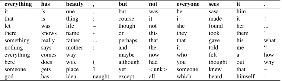
-Table 4: Ten most probable word substitutions on each position in the sentence ”Everything has beauty, but not everyone sees it.” produced by 1000 roles LTLM with the deterministic inference.
cantly outperformed STLM where the syntactic de-pendency trees were provided as a prior knowledge. The joint learning of syntax and semantics of a sen-tence proved to be more suitable for predicting the words.
An in-depth analysis of semantic and syntactic properties of LTLM is beyond the scope of this pa-per. For better insight into the behavior of LTLM, we show the most probable word substitutions for one selected sentence (see Table 4). We can see that the original words are often on the front po-sitions. Also it seems that LTLM is more syntac-tically oriented, which confirms claims from (Levy and Goldberg, 2014; Pad´o and Lapata, 2007), but to draw such conclusions a deeper analysis is required. The properties of the model strongly depends on the number of distinct roles. We experimented with maximally 1000 roles. To catch the meaning of var-ious words in natural language, more roles may be needed. However, with our current implementation, it was intractable to train LTLM with more roles in a reasonable time. Training 1000 roles LTLM took up to two weeks on a powerful computational unit.
7 Conclusion and Future Work
In this paper we introduced the Latent Tree Lan-guage Model. Our model discovers the latent tree structures hidden in natural text and uses them to predict the words in a sentence. Our experiments with English and Czech corpora showed dramatic improvements in the predictive ability compared with standalone Modified Kneser-Ney LM. Our Java implementation is available for research purposes at
https://github.com/brychcin/LTLM.
It was beyond the scope of this paper to explic-itly test the semantic and syntactic properties of the model. As the main direction for future work we plan to investigate these properties for example by comparison with human-assigned judgments. Also, we want to test our model in different NLP tasks (e.g. speech recognition, machine translation, etc.).
We think that the role-by-role distribution should depend on the distance between the parent and the child, but our preliminary experiments were not met with success. We plan to elaborate on this assump-tion. Another idea we want to explore is to use different distributions as a prior to multinomials. For example, Blei and Lafferty (2006) showed that the logistic-normal distribution works well for topic modeling because it captures the correlations be-tween topics. The same idea might work for roles.
Acknowledgments
This publication was supported by the project LO1506 of the Czech Ministry of Education, Youth and Sports. Computational resources were provided by the CESNET LM2015042 and the CERIT Sci-entific Cloud LM2015085, provided under the pro-gramme ”Projects of Large Research, Development, and Innovations Infrastructures”. Lastly, we would like to thank the anonymous reviewers for their in-sightful feedback.
References
[image:9.612.74.541.57.191.2]lan-guage model. Journal of Machine Learning Research, 3:1137–1155, March.
David M. Blei and John D. Lafferty. 2006. Correlated topic models. InIn Proceedings of the 23rd Interna-tional Conference on Machine Learning, pages 113– 120. MIT Press.
Ondˇrej Bojar, Zdenˇek ˇZabokrtsk´y, Ondˇrej Duˇsek, Pe-tra Galuˇsˇc´akov´a, Martin Majliˇs, David Mareˇcek, Jiˇr´ı Marˇs´ık, Michal Nov´ak, Martin Popel, and Aleˇs Tam-chyna. 2012. The joy of parallelism with czeng 1.0. InProceedings of the Eight International Conference on Language Resources and Evaluation (LREC’12), Istanbul, Turkey, may. European Language Resources Association (ELRA).
Peter F. Brown, Peter V. deSouza, Robert L. Mercer, Vin-cent J. Della Pietra, and Jenifer C. Lai. 1992. Class-based n-gram models of natural language. Computa-tional Linguistics, 18:467–479.
Tom´aˇs Brychc´ın and Miloslav Konop´ık. 2014. Semantic spaces for improving language modeling. Computer Speech & Language, 28(1):192–209.
Tom´aˇs Brychc´ın and Miloslav Konop´ık. 2015. Latent semantics in language models. Computer Speech & Language, 33(1):88–108.
Stanley F. Chen and Joshua T. Goodman. 1998. An empirical study of smoothing techniques for language modeling. Technical report, Computer Science Group, Harvard University.
Shay B. Cohen, Kevin Gimpel, and Noah A. Smith. 2009. Logistic normal priors for unsupervised prob-abilistic grammar induction. In Advances in Neural Information Processing Systems 21, pages 1–8. Arthur P. Dempster, N. M. Laird, and D. B. Rubin. 1977.
Maximum likelihood from incomplete data via the em algorithm. Journal of the Royal Statistical Society. Se-ries B, 39(1):1–38.
Koen Deschacht, Jan De Belder, and Marie-Francine Moens. 2012. The latent words language model.
Computer Speech & Language, 26(5):384–409. Zellig Harris. 1954. Distributional structure. Word,
10(23):146–162.
William P. Headden III, Mark Johnson, and David Mc-Closky. 2009. Improving unsupervised dependency parsing with richer contexts and smoothing. In Pro-ceedings of Human Language Technologies: The 2009 Annual Conference of the North American Chapter of the Association for Computational Linguistics, pages 101–109, Boulder, Colorado, June. Association for Computational Linguistics.
Sandra K¨ubler, Ryan McDonald, and Joakim Nivre. 2009. Dependency parsing. Synthesis Lectures on Hu-man Language Technologies, 2(1):1–127.
Martin Lange and Hans Leiß. 2009. To cnf or not to cnf? an efficient yet presentable version of the cyk algorithm.Informatica Didactica, 8.
Omer Levy and Yoav Goldberg. 2014. Dependency-based word embeddings. InProceedings of the 52nd Annual Meeting of the Association for Computational Linguistics (Volume 2: Short Papers), pages 302–308, Baltimore, Maryland, June. Association for Computa-tional Linguistics.
David Mareˇcek and Milan Straka. 2013. Stop-probability estimates computed on a large corpus im-prove unsupervised dependency parsing. In Proceed-ings of the 51st Annual Meeting of the Association for Computational Linguistics (Volume 1: Long Papers), pages 281–290, Sofia, Bulgaria, August. Association for Computational Linguistics.
Sven Martin, Jorg Liermann, and Hermann Ney. 1998. Algorithms for bigram and trigram word clustering.
Speech Communication, 24(1):19–37.
Ryan McDonald, Fernando Pereira, Kiril Ribarov, and Jan Hajiˇc. 2005. Non-projective dependency parsing using spanning tree algorithms. InProceedings of the Conference on Human Language Technology and Em-pirical Methods in Natural Language Processing, HLT ’05, pages 523–530, Stroudsburg, PA, USA. Associa-tion for ComputaAssocia-tional Linguistics.
Tom´aˇs Mikolov, Martin Karafi´at, Luk´aˇs Burget, Jan ˇCernock´y, and Sanjeev Khudanpur. 2010. Recurrent neural network based language model. InProceedings of the 11th Annual Conference of the International Speech Communication Association (INTERSPEECH 2010), volume 2010, pages 1045–1048. International Speech Communication Association.
Tom´aˇs Mikolov, Stefan Kombrink, Luk´aˇs Burget, Jan ˇCernock´y, and Sanjeev Khudanpur. 2011. Exten-sions of recurrent neural network language model. InProceedings of the IEEE International Conference on Acoustics, Speech, and Signal Processing, pages 5528–5531, Prague Congress Center, Prague, Czech Republic.
Thomas P. Minka. 2003. Estimating a dirichlet distribu-tion. Technical report.
Sebastian Pad´o and Mirella Lapata. 2007. Dependency-based construction of semantic space models. Compu-tational Linguistics, 33(2):161–199, June.
Martin Popel and David Mareˇcek. 2010. Perplex-ity of n-gram and dependency language models. In
Proceedings of the 13th International Conference on Text, Speech and Dialogue, TSD’10, pages 173–180, Berlin, Heidelberg. Springer-Verlag.
improves unsupervised dependency parsing. In Pro-ceedings of the Fourteenth Conference on Computa-tional Natural Language Learning, pages 9–17, Up-psala, Sweden, July. Association for Computational Linguistics.
Valentin I. Spitkovsky, Hiyan Alshawi, Angel X. Chang, and Daniel Jurafsky. 2011. Unsupervised dependency parsing without gold part-of-speech tags. In Proceed-ings of the 2011 Conference on Empirical Methods in Natural Language Processing, pages 1281–1290, Ed-inburgh, Scotland, UK., July. Association for Compu-tational Linguistics.