LEABHARLANN CHOLAISTE NA TRIONOIDE, BAILE ATHA CLIATH TRINITY COLLEGE LIBRARY DUBLIN OUscoil Atha Cliath The University of Dublin
Terms and Conditions of Use of Digitised Theses from Trinity College Library Dublin
Copyright statement
All material supplied by Trinity College Library is protected by copyright (under the Copyright and Related Rights Act, 2000 as amended) and other relevant Intellectual Property Rights. By accessing and using a Digitised Thesis from Trinity College Library you acknowledge that all Intellectual Property Rights in any Works supplied are the sole and exclusive property of the copyright and/or other I PR holder. Specific copyright holders may not be explicitly identified. Use of materials from other sources within a thesis should not be construed as a claim over them.
A non-exclusive, non-transferable licence is hereby granted to those using or reproducing, in whole or in part, the material for valid purposes, providing the copyright owners are acknowledged using the normal conventions. Where specific permission to use material is required, this is identified and such permission must be sought from the copyright holder or agency cited.
Liability statement
By using a Digitised Thesis, I accept that Trinity College Dublin bears no legal responsibility for the accuracy, legality or comprehensiveness of materials contained within the thesis, and that Trinity College Dublin accepts no liability for indirect, consequential, or incidental, damages or losses arising from use of the thesis for whatever reason. Information located in a thesis may be subject to specific use constraints, details of which may not be explicitly described. It is the responsibility of potential and actual users to be aware of such constraints and to abide by them. By making use of material from a digitised thesis, you accept these copyright and disclaimer provisions. Where it is brought to the attention of Trinity College Library that there may be a breach of copyright or other restraint, it is the policy to withdraw or take down access to a thesis while the issue is being resolved.
Access Agreement
By using a Digitised Thesis from Trinity College Library you are bound by the following Terms & Conditions. Please read them carefully.
TRINITY c o l l e g e' 21
\m M L
Iter a tiv e T h ree -D im en sio n a l H e lm h o ltz E q u a tio n
S o lu tio n s u sin g th e W ave E x p a n sio n M e th o d
B harath Gopalaswamy
A thesis subm itted to the University of D ubhn in partial fulfilment of the requirements for the degree of
D o c to r o f P h ilo s o p h y
D epartm ent of Mechanical and M anufacturing Engineering, Trinity College Dublin,
D e c la r a tio n
I hereby declare th a t my thesis has not been previously subm itted as an exercise for a degree at this or any other university. Except where otherwise acknowledged, the research is entirely the work of the author. Permission is granted for the library of Trinity College Dublin to lend or copy this thesis upon request.
C .
B
B harath Gopalaswamy, Trinity College Dublin,
Su m m ary
Modelling sound propagation often can present difficult challenges due to compu tational demands. In general, the direct solutions of the system equations arising from the full field discretization of many three-dimensional problems of practical engineering interest cannot be attem pted. The current study consists of modelling sound propagation through a full field approach known as the Wave Expansion M ethod (W EM ). The boundary conditions used in this study are Neumann and Free radiation conditions. The m ajor advantage of the WEM is th a t it requires only around 2-3 nodes per wavelength to obtain accurate solutions which oflfers a sig nificant com putational advantage over conventional finite element, finite difference and boundary element approaches, which require around 8-10 nodes per wavelength.
A central question which arises using the WEM concerns the m aintenance of ade quate convergence under an iterative solver since any numerical discretization pro cedure is rendered incomplete w ithout a proper solution procedure. The present study comprises a thorough investigation into standard Krylov sub-space iterative solvers and examines its suitability to the WEM.
Successful com putations over large systems using the standard BI-CGSTAB and the restarted versions of the GMRES algorithm on a P-IV, 882 Mb RAM, 2.2 GHz machine were carried out. The W EM models are found to behave well with both th e BI-CGSTAB and the restarted versions of GMRES. However, BI-CGSTAB was preferred because of its lower memory requirements during iterations as compared to GMRES.
The effects of preconditioning were analyzed in the system and it was found th a t the ILUT and Jacobi preconditioners do not affect the convergence of the numeri cal systems when the models are discretized with around 3 nodes per wavelength. However, when the models were discretized with around 7 nodes per wavelength, the ILUT preconditioner dram atically improved the convergence in the case of models discretized with structured hexahedral elements. In the case of tetrahedral elements, the preconditioner still had no effect.
A cknow ledgm ents
I gratefully acknowledge that this thesis would not have been possible without the
financial assistance of the EU-FP6 NACRE Project contract no:
AIPA
— C T —
2005 - 516068.I would like to thank Prof. Henry Rice, my research supervisor, for his guidance,
patience, knowledge and skill without which the work in this thesis would not have
been possible.
I am also indebted to Hugh Hill for being such a good friend and a great advisor.
Hugh supported me through out this work and constantly encouraged me.
I would also like to thank and acknowledge the help of Joan, the departmental ex
ecutive officer, and all the technicians of the Mechanical Engineering Department
for their assistance along the way.
This thesis owes much to all those people who enriched me with their friendship during my time in Dublin. Special thanks to P altu (Titiksh Patel), and gunda (Deepak). They have been a great source of support and their constant encourage m ent helped me get through my toughest times.
To my “m ates” at th e office: Diego (Leandro) for his support, useful discussions and ideas, E nda for his singing th a t provided the necessary entertainm ent, Ciaran for his support, and his help with M atlab, Jens for the useful discussions. To the “lads” in the “ex-upper seminar room” : Bjorn, Stephen, Cathal, Eoin and John, and to all the postgraduates students in the MME D epartm ent.
I would like to dedicate this thesis to my family for the love and support they have given me throughout my life.
B HA RATH GoPA L A SW A M Y
C ontents
S u m m a ry ii
A c k n o w le d g m e n ts iv
L ist o f T ables x
L ist o f F igu res xiii
C h a p ter 1 In tr o d u ctio n 1
1.1 M otivation; G eneral E ngineering In terest ... 1
1.2 Definition of A coustic P r o b le m s ... 3
1.3 Review of Num erical M ethods applicable to Acoustic problem s . . . 3
1.3.1 F inite Elem ent M ethod ... 4
1.3.2 F inite Difference M e t h o d s ... 5
1.3.3 B oundary Elem ent M e t h o d ... 5
1.3.4 W^ve Expansion M ethod ... 6
1.4 C om putational C o s t ... 7
1.5 S tru ctu re of th e T h e s is ... 8
2.2 Direct S o lv e rs ... 11
2.3 Iterative Solvers ... 15
2.3.1 Introduction ... 15
2.3.2 Basic Iterative M e t h o d s ... 16
2.3.3 Stationary M ethods ... 16
2.3.4 N on-stationary methods- Krylov Subspace M e t h o d s ... 18
2.3.5 Conjugate G radient Squared M e th o d ... 19
2.3.6 Bi-Conjugate G radient Stabilization, B i- C G S T A B ... 21
2.3.7 Generalized Minimal Residual-(GM RES) ... 24
2.4 M ultigrid Approaches ... 26
2.4.1 Domain Decomposition ... 31
2.5 D iscu ssio n ... 36
C h a p te r 3 I m p le m e n ta tio n o f th e N u m e r ic a l S y s t e m 38 3.1 In tro d u c tio n ... 38
3.2 Wave Expansion M e th o d ... 39
3.2.1 Wave Expansion M ethod- F o rm u la tio n ... 40
3.2.2 Boundary Conditions ... 41
3.2.3 Algorithmic Implementation of the Wave Expansion Method 44 3.3 Solution Techniques for the Wave Expansion M e th o d ... 45
3.4 Wave Expansion M ethod-Implementation on structured meshes . . . 46
3.4.1 Numerical Results for structured elements using Bi-CGSTAB 46 3.4.2 Numerical Results for structured liexahedral elements using G M R E S ... 54
3.4.3 Implementation of the WEM on U nstructured Meshes . . . . 59
3.5 D iscu ssio n ... 68
C h a p te r 4 R e v ie w a n d I m p le m e n ta t io n o f P r e c o n d itio n e r s 76 4.1 P re c o n d itio n e rs... 76
4.1.1 Introduction ... 76
4.2 Qualities of a good preconditioner ... 77
4.3 Jacobi Preconditioner ... 78
4.3.1 Block Jacobi M e th o d s ... 79
4.3.2 Numerical Simulations- Jacobi P re c o n d itio n e rs ... 79
4.4 Incomplete Factorization Preconditioners ... 81
4.4.1 Incomplete Factorization A lg o rith m s ... 81
4.4.2 Drop Tolerance in the usage of P re c o n d itio n e rs ... 82
4.4.3 Numerical simulations using ILUT- Dual Threshold Strategy P r e c o n d itio n e r ... 83
4.5 Eigenvalue Analysis ... 89
4.5.1 Problem discretized with hexahedral meshes, {ppw ~ 3) . . . 89
4.5.2 Problems discretized with hexahedral meshes, (ppu> ~ 7) . . . 93
4.5.3 Problems discretized with tetrahedral meshes, {ppw ~ 3) . . . 97
4.5.4 Problem s discretized with tetrahedral meshes, {ppw ~ 7) . . . 101
4.6 Additive Schwarz Preconditioning M e t h o d s ...105
4.6.1 Preconditioning A p p ro a c h ... 106
4.6.2 Numerical S im u latio n s...107
4.7 D iscu ssion...108
5.3 Noise Shielding Effect by an High-Lift Device as a w i n g ... 115 5.4 The Effect of the S c a tte re r... 120 5.5 D iscu ssio n ... 122
C h a p te r 6 C o n c lu s io n s 123
6.1 C o n c lu sio n s ... 123 6.2 F uture Work ... 125
List of Tables
2.1 D ir e c t S o lv er in T w o - D i m e n s i o n s ... 13 2.2 D ir e c t S o lv er in T h r e e - D i m e n s i o n s ... 14 2.3 P e r f o r m a n c e o f t h e m u ltig r id a p p r o a c h fo r a s e t o f p ro b le m s
in t w o - d i m e n s i o n s ... 29
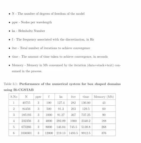
3.1 P e rfo rm a n c e o f t h e n u m e ric a l s y s te m fo r b o x s h a p e d d o
m a in s u sin g B i-C G S T A B 49
3.2 P e rfo rm a n c e o f th e n u m e ric a l s y s te m fo r b o x s h a p e d d o m a in s u sin g G M R E S r e s t a r t = 5 54 3.3 P e rfo rm a n c e o f th e n u m e ric a l s y s te m fo r b o x s h a p e d ....d o
m a in s u sin g G M R E S r e s t a r t = 6 54 3.4 P e rfo rm a n c e o f th e n u m e ric a l s y s te m fo r b o x s h a p e d ... d o
m a in s u sin g G M R E S r e s t a r t = 7 55 3.5 P e r f o r m a n c e o f t h e n u m e ric a l s y s te m fo r b o x s h a p e d d o
m a in s u sin g G M R E S r e s t a r t = 8 55 3.6 P e r f o r m a n c e o f th e n u m e ric a l s y s te m fo r b o x s h a p e d ... d o
m a in s u sin g G M R E S r e s t a r t = 9 56 3.7 P e r fo rm a n c e o f th e n u m e ric a l s y s te m fo r s c a tt e r in g p r o b
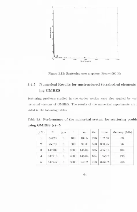
3.8 P e r f o r m a n c e o f th e n u m e ric a l s y s te m for s c a tte r in g p r o b le m s u s in g G M R E S ( r ) = 5 ... 64 3.9 P e r f o r m a n c e o f th e n u m e ric a l s y s te m fo r s c a tte r in g p r o b
le m s u s in g G M R E S ( r ) = 6 ... 65 3.10 P e r f o r m a n c e o f th e n u m e ric a l s y s te m fo r s c a tte r in g p r o b
le m s u s in g G M R E S ( r ) = 7 ... 65 3.11 P e r f o r m a n c e o f th e n u m e ric a l s y s te m fo r s c a tte r in g p r o b
le m s u s in g G M R E S ( r ) = 8 ... 65 3.12 P e r f o r m a n c e o f th e n u m e ric a l s y s te m for s c a tte r in g p r o b
le m s u s in g G M R E S ( r ) = 9 ... 66 3.13 C o m p u ta tio n a l e ffo rt fo r p ro b le m s w ith , ka = 146.04 ... 70
4.1 P e r f o r m a n c e o f th e n u m e ric a l s y s te m for b o x s h a p e d d o m a in s u s in g B i-C G S T A B w ith J a c o b i p r e c o n d itio n e r s . . . . 80 4.2 P e r f o r m a n c e o f th e n u m e ric a l s y s te m fo r b o x s h a p e d d o
m a in s u s in g B i-C G S T A B w ith o u t th e p r e c o n d itio n e r . . . . 80 4.3 P e r f o r m a n c e o f th e n u m e ric a l s y s te m for b o x s h a p e d d o
m a in s u s in g B i-C G S T A B w ith IL U T P r e c o n d i t i o n e r ... 86 4.4 E x tr e m e e ig e n v a lu e s a n d c o n d itio n in g in f o r m a tio n o f th e
m a t r i x ... 90 4.5 E x t r e m e e ig e n v a lu e s a n d c o n d itio n in g in f o r m a tio n o f th e
m a t r i x ... 94 4.6 E x tr e m e e ig e n v a lu e s a n d c o n d itio n in g in f o r m a tio n o f th e
m a t r i x ... 98 4.7 E x tr e m e e ig e n v a lu e s a n d c o n d itio n in g in f o r m a tio n o f th e
5.1 P e r f o r m a n c e o f th e n u m e ric a l s y s te m ... 115
5.2 P e r f o r m a n c e o f th e n u m e ric a l s y s te m ... 118
5.3 In flu e n c e o f t h e S c a t t e r e r ... 121
List o f Figures
2.1 Real p art of pressure obtained by scattering over an a irfo il... 14
2.2 Schematic representation of a V-cycle m u ltig rid ... 27
2.3 Real p art of pressure on a box shaped domain using the multigrid ap p ro ac h ... 30
2.4 Basic idea of the additive Schwarz i t e r a t i o n ... 33
2.5 Basic idea of the multiplicative Schwarz it e r a t i o n ... 34
3.1 N atural Radiation Boundary Condition Im p le m e n ta tio n ... 42
3.2 Schematic representation of the p r o b le m ... 47
3.3 Sparsity P attern of the stiffness m atrix (Number of non-zeros=17757796) 48 3.4 Real P art of Pressure on a box shaped domain ... 51
3.5 Sound Pressure Levels on a box shaped d o m a in ... 52
3.6 Convergence graph for the numerical s y s te m ... 53
3.7 Real p art of pressure obtained on a box shaped domain by GMRES 57 3.8 SPL (dB) obtained on a box shaped domain by GMRES, r= 7 . . . . 58
3.9 Convergence graph for the numerical sj^stem ... 59
3.10 Sparsity p a tte rn of the stiffness m atrix (Number of non-zeros=8027565) 60 3.11 Schematic representation of the p r o b le m ... 62
3.12 Scattering over a sphere, Freq=4000 H z ... 63
3.14 Real p art of pressure for scattering over a sphere using GMRES (r)=9,
Freq=4000 H z ... 67
3.15 Performance of the Numerical system using the GMRES (r)=9 . . . 68
3.16 Sparsity p attern with a re-ordered s c h e m e ... 72
3.17 Sparsity p attern with the re-ordered scheme for a reduced m atrix . . 73
3.18 Sparsity pattern with the re-ordered scheme for a m atrix with trian gular elements ... 74
3.19 Sparsity p attern with the re-ordered scheme for a reduced m atrix . . 75
4.1 Sparsity pattern of the original stiffness m a t r i x ... 84
4.2 Sparsity p attern of the stiffness m atrix w ith r = 4 e — 1 ... 85
4.3 Real P art of pressure for a box shaped domain, Freq= 8000 Hz . . . 87
4.4 SPL (dB) of a box shaped domain using a preconditioner, Freq= 8000 H z ... 88
4.5 Eigenvalues of the co-efficient m a t r i x ... 91
4.6 Eigenvalues of the m atrix preconditioned w ith I L U T ... 92
4.7 Eigenvalues of the m atrix with Jacobi P re c o n d itio n in g ... 93
4.8 Eigenvalues of the original m a tr ix ... 95
4.9 Eigenvalues of the m atrix with Jacobi p re c o n d itio n e r... 96
4.10 Eigenvalues of the m atrix with ILUT p r e c o n d itio n e r ... 97
4.11 Eigenvalues of the original m a tr ix ... 99
4.12 Eigenvalues of the Jacobi preconditioned m atrix ...100
4.13 Eigenvalues of the m atrix preconditioned with I L U T ... 101
4.14 Eigenvalues of the original m a tr ix ... 103
4.15 Eigenvalues of the m atrix preconditioned with I L U T ...104
4.16 Eigenvalues of the m atrix with a Jacobi p reco n d itio n e r...105
5.2 Acoustics Pressure Field for Tank, Freq=200 Hz ... 114
5.3 Schematic representation of a shielding effect p r o b l e m ... 116
5.4 Sparsity p attern of a stiffness m atrix, nnz=9449026 ... 117
5.5 Shielding Effect by an Aircraft High Lift D e v ic e ... 119
C hapter 1
In trod u ction
This thesis investigates iterative solution techniques for wave problems occurring in three-dimensions. The Hemholtz equation which represents the wave propagation in the frequency-domain is used to model the wave problems studied in this thesis.
The Helmholtz equation finds its use in many scientific areas such as the acoustic phenomena occurring with the aircraft [1], underw ater acoustics applications [2, 3, 4], geo-physical applications [5, 6] and electromagnetic applications [7, 8]. In this thesis, the focus of the applications is on general engineering applications and applications in the acoustic phenomena occurring with aircraft.
1.1
M otiv a tio n : G en eral E n g in eerin g In terest
perturbation, and there are numerous methods available to solve the Poisson’s equa tion. However, this perturbation, which shows up as the extra term in the Helmholtz equation is the source of all complications and proposes a lot of difficulty when one attem p ts to solve it iteratively.
A considerable am ount of research has been done in the recent years to find an efficient solution for the Helmholtz equation. Bayliss et. al [9] provided an efficient im plem entation of an iterative scheme by using the conjugate gradient m ethod and this paper can be considered as one of the earliest in this area. Further work was done in contributions [10, 11]. However, all these works w'ere quite ineffective in term s of efficiency for solving problems with high Helmholtz numbers.
An ideal solver for the Helmholtz equation should be capable of dealing with prob lems with high Helmholtz number, which is defined as follows:
Hji = ka (1-1)
1.2
D e fin itio n o f A c o u stic P ro b lem s
The propagation of acoustic waves is given by the general wave equation [13]
=
(1.2)
where c is the sound speed and p{x, t) is the acoustic pressure at time t and position X .
For modelling purposes, the use of Eq. 1.2 requires not only a spatial discretization but also a tim e step discretization. An im portant simplification in the formulation is obtained if only the steady-state harmonic pressure p{x) is considered. Eq. 1.2 then reduces to ’’Helmholtz E quation” , m athem atically expressed as
V^p(x) + /c^p(x) = 0 (1.3)
The ratio k = uj/c is the wavenumber and w=2irf where / is the signal frequency. The performance of the numerical method is often assessed by the number of nodes per wavelength required by the discretization to produce accurate results. The number of nodes per wavelength is given by Eq. 1.4
ppw = c / h . f (1-4)
where h is the minimum nodal spacing in the mesh.
1.3
R e v ie w o f N u m erica l M e th o d s a p p lica b le to A c o u s
tic p rob lem s
introduction to th e wave expansion m ethod (WEM), which is prim arily a highly efficient wave based finite difference scheme.
The FE and FD are full field discretization techniques unlike the BE m ethods in which the discretization is performed only in the boundary of the com putational domain. Commercially available tools are usually a variant of the stand ard finite element (FE), finite difference (FD), boundary element (BE) methods. Sections 1.3.1, 1.3.2 and 1.3.3 provide a brief review of the numerical techniques.
1.3 .1
F in ite E le m en t M e th o d
The finite element method is one of the most common m ethods and is probably the most widely used m ethod in the numerical modelling of problems of general engineering interest due to its adaptability and straightforward implem entation. The m ethod is based on the following concepts
• transform ation of the original differential problem to its respective integral formulation.
• division of the continuum into smaller non-overlapping sub domains called elements over which th e system integral equations may be summed.
• approxim ation of the field variable distributions and the geometry and the geom etry of the continuum domain, in term s of a set of shape functions, which are locally defined in each element.
For a detailed description about the finite element m ethod and its application to solving acoustic problems, the reader is referred to [14, 15].
1 .3 .2
F in ite D iffer en ce M e th o d s
The finite difference m ethod (FDM) like the finite element is a full-field discretization technique and is also a popular technique to model the Helmholtz problem. The basic principles of the finite difference method are :
• discretization of th e domain into a finite number of points uniformly dis trib u ted within th e domain
• approxim ation of the derivatives of the governing equation by interpolating polynomials, formulated in term s of surrounding points in the grid
• solution of a system of equations of the form A x = b, where x is the field variable approxim ated field variable at each discretization point, and A is the banded m atrix formed by the mass, stiffness and dam ping matrices.
For a detailed description about the finite difference m ethod and its application in solving acoustic problems, the reader is referred to [16, 17]
1 .3 .3
B o u n d a ry E le m e n t M e th o d
offset by the full structure of the system m atrix which means th a t an iterative full field m ethod in three-dimensions may be still be more com putationally efficient.
There are two main approaches in obtaining the boundary integral equation formu lation for acoustic problems. The first m ethod is the so-called ’’direct m ethod’' and the second m ethod is the ’’indirect boundary element m ethod” . However, based on the direct or indirect formulation, the boundary element solution is obtained by the following procedure:
• The field equations are transform ed to a boundary integral using the diver gence theorem.
• The boundary is discretized and the integral is formulated using the loading points on the boundary.
• A full system equation of the form A x = / results, which yields acoustic pressure values at the boimdary.
For a detailed description of the BEM and their formulation for acoustic problems, the reader is referred to [18, 19, 20, 21]
1 .3 .4
W ave E x p a n sio n M e th o d
and unstructured meshes [23]. A detailed description regarding the implem entation of the WEM is provided in C hapter 3.
1.4
C om putational Cost
A brief comparison of com putational cost associated with full field m ethods such as FEM , FDM is made with the BEM in three-dimensions.
of memory and potentially reduce com putational loading in term s of calcula tions from o{ N ‘^) to o(A^^ log A^^). However, convergence of any iterative solutions still must be ensured in order employ any of th e above methods. In addition, the foregoing discussion is also dependent on the relative size of the scatterer within the meshed domain.
1.5
S tru ctu re o f th e T h esis
C hapter Two gives a review of the solution techniques applicable to the solution of the Helmholtz equation. A description of the Krylov subspace solvers th a t are used in this study is provided. The chapter also provides a review of the multigrid and domain decomposition techniques th a t could effectively be used to obtain the solutions of the Helmholtz equations.
C hapter Three is concerned with the im plem entation of the wave expansion method. The formulation, the methodology and the im plem entation of the W EM and the boundary conditions are also discussed. Furtherm ore, the discretization on both structured and unstructured meshes are studied with respect to obtaining solutions with standard krylov sub-space solvers.
Chapter Five presents two practical applications of the W EM model to examine its suitability to real scale engineering problems while
C h a p ter 2
R ev iew o f N u m erical solu tion
tech n iq u es applicable to
H elm h oltz eq u ation
2.1
I n t r o d u c t io n
For most acoustic problems, the solution of the partial differential equations can not be found in closed analytical form mainly due to complex geometry and the boundary conditions [24, 25]. Therefore, an approxim ation of the exact solution is searched for by transform ing the m athem atical model into a set of algebraic equa tions th a t are amenable to numerical solution procedures. The equations generally result in the form
A x = b (2.1)
being addressed in this thesis is fully three-dimensional, any discretization would result in a large number of unknowns and this results in a considerable amount of com putational storage space being utilized. Three Dimensional problems also gen erate m atrix equations with high bandwidth.
Direct m ethods based on Gaussian elimination with partial pivoting require pro hibitive am ount of additional storage, thus imposing a demand for iterative methods the most advanced of which are the Krylov sub-space m ethods [26, 27, 28, 29]. This chapter aims at providing a brief insight into some of the existing solvers th a t are useful in providing solutions to the Helmholtz equation.
2.2
D irect Solvers
Any m athem atical model gives rise to a large linear system of algebraic equation. One of the most common methods th at is based on factorization of the m atrix in triangular factors is known as the ”LU Decomposition” approach [30]. In this approach, the co-efficient m atrix is factorized into the product of a lower triangular m atrix, L and a upper triangular m atrix, U such th at
A = LU (2.2)
The solution then can be easily obtained by solving two triangular systems
Ly = b (2.3)
and
Ux = y (2.4)
the triangular matrices, L and U due to the high bandw idth of the original m atrix A.
Direct methods, based on the above factorization are usually the choice in many codes where problem sizes are small enough so th a t the storage requirem ent do not exceed the available capacity. This is primarily due to their robustness and their predictabihty in term s of time and storage required for com putation. Modern day solvers have m ade it possible to efficiently solve fairly large linear systems in a reasonable am ount of tim e particularly when the problem is two-dimensional. For a system of linear equations with m oderate dimension, the solution is and can be obtained by using direct solvers. Direct solvers give exact solutions except for rounding-off errors, which may arise due to the o(L^) where b is the bandw idth of the m atrix, operations required. However, when the number of equations becomes large, the use of iterative solvers becomes unavoidable.
As mentioned in th e earlier chapter, three-dimensional problems generate system matrices with higher bandw idth relative to the row count compared to two-dimensional problems.
As a result, direct solvers suffer from poor scalability with respect to operation counts and memory requirements of problems arising from th e discretization of P D E ’s from three-dimensional systems [31].
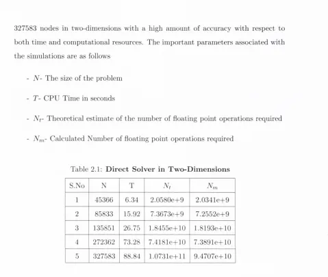
A set of problems using direct solvers in two and three-dimensional problems have been presented in Table 2.1 and Table 2.2. The problems studied here are discretized using the Wave Expansion M ethod. The com putations were performed on an IBM, Pentium -IV machines with 882 MB of RAM and a clock speed of 2.2 Ghz.
327583 nodes in two-dimensions with a high amount of accuracy with respect to both tim e and com putational resources. The im portant param eters associated with the sinm lations are as follows
- TV- The size of the problem
- T- CPU Time in seconds
- Nf- Theoretical estim ate of the number of floating point operations required
- Nm- Calculated Number of floating point operations required
Table 2.1; D irect Solver in T w o -D im en sio n s
S.No N T Nt iVm
1 45366 6.34 2.0580e+9 2.0341e-F9
2 85833 15.92 7.3673e-^9 7.2552e-K9 3 135851 26.75 1.8455e+10 1.8193e-hl0 4 272362 73.28 7.4181e-f-10 7.3891e+10
5 327583 88.84 1.0731e+ll 9.4707e-hl0
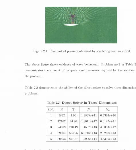
[image:31.547.53.532.50.455.2]Figure 2.1: Real p art of pressure obtained by scattering over an airfoil
The above figure shows evidence of wave behaviour. Problem no.5 in Table 2.1 dem onstrates the am ount of com putational resources required for the solution of the problem.
Table 2.2 dem onstrates the ability of the direct solver to solve three-dimensional problems.
Table 2.2: D ir e c t S o lv er in T h re e -D im e n s io n s
S.No N T
Nt
Nrr,
1 5832 4.96 1.9835e-^ll 6.6324e-f-10 2 12167 44.96 1.8011e-M2 6.0127e-hll 3 24389 210.49 1.4507e-hl3 4.8393e-M2 4 39304 664.95 6.0716e-hl3 2.0248e-M3 5 50653 877.57 1.2996e-hl4 4.3336e-hl3
[image:32.547.19.493.56.580.2]point operations and the measured floating point operations.
Three-dimensional problems clearly require extensive com putational resources and it is quite impossible to solve problems arising from discretization of really large engineering systems of practical interest by direct solvers. Hence, it is imperative to resort to iterative solvers.
2.3
Itera tiv e Solvers
2.3.1
I n tr o d u c tio n
Iterative methods can be classified into two groups, stationary and non-stationary methods. Stationary methods refer to classical iterative methods such as Jacobi, Gauss-Seidel and SSOR [32]. The non-stationary methods can be classified as Krylov sub-space methods such as the Conjugate G radient Squared (CCS) [39], generalized minimal residual (GMRES) [33], bi-conjugate gradient (Bi-CG) and bi-conjugate gradient stabilized (Bi-CGStab) [34].
This chapter does not aim at providing an exhaustive review of every possible itera tive solvers th a t may be used for acoustic problems. The discussion in this chapter is centered around the standard non-stationary iterative solvers th a t have been devel oped, investigated and tested for acoustic problems. The latter p art of the chapter also discusses multigrid approaches and domain decomposition algorithms, which have been studied for solving large acoustics problems arising out of the discretiza tion of the helmholtz equation.
converge and can often take a significant more time th an direct solvers subject to memory availability. However, this particular phenomenon can, in principle, be im proved by the use of another m atrix known as the preconditioner, which is discussed in detail in C hapter 4.
The following sections provide a brief review of some of the standard iterative solvers th a t have been used for solving large linear system of equations.
2 .3 .2
B a sic I te r a tiv e M e th o d s
Iterative m ethods are usually of two types: stationary and non-stationary methods. S tationary m ethods are usually simpler, easier to understand and implement when com pared to non-stationary methods. However, they are generally less as effective and probably of little value when attem pting solutions of the Helmholtz equation, which is poorly conditioned at high ”ka” values [10]. On the other hand, non- stationary m ethods are a relatively recent development, more difficult to understand but can be very effective. The subsequent sections explore the methods in more detail.
2 .3 .3
S ta tio n a r y M e th o d s
Consider a basic splittingA = U - G , U , G (2.5)
where N is the number of unknowns. By substituting Eq. 2.5into Eq.2.1 we obtain
{ U - G ) u = g < ^ U u = g + Gu (2.6)
approxima-tion can be computed as
Uu^ = g + Gu^-^ ^ = U - \ g + Gu^~^) (2.7)
Thus,
u J = U-^g + (I - U- ^A) u ^- ^
^ ^ (2.8)
=
with — l'.=g — Au^~^ the residual after the (j — 1)^^ iteration, and I the identity m atrix. Equation 2.8 is defined as the basic iterative method. The way in which the splitting is chosen primarily distinguishes the basic iteration strategy. The m atrix A could be decomposed in the following way
A = D - E - U (2.9)
where
- —D the diagonal
- —E the strictly lower triangular part of A
- —U the strictly upper triangular p art of A
In the Jacobi method, A = D — E \s chosen and the iteration is carried out as follows
(2-10)
By splitting A = L — U, the Gauss-Seidel iteration is obtained, where L and U are the upper and lower triangular matrices, respectively. The resulting iteration is w ritten as follows
By extrapolating th e Gauss-Seidel Method, the Successive Overrelaxation Method, or SOR can be devised. The extrapolation takes the form of a weighted residual approach between the previous iterate and the com puted Gauss-Seidel iterate suc cessively for each component as follows
+ { 1 - (2.1 2)
where {x denotes a Gauss-Seidel iterate , and is the relaxation factor). The basic idea here is to choose an optim al value for /i th a t will enhance the rate of convergence of the iterates to the solution. In m atrix terms, the SOR equation can be w ritten as follows:
xW = { D - + {iiU + (1 - ^l)D)x^^-^'^ + fi{D - (2.13)
The pseudo-code for the SOR can be found in [32]. Further developments on the SOR involve the optim ization of the relaxation factor
2 .3 .4
N o n -s ta tio n a r y m e th o d s- K r y lo v S u b sp a c e M e th o d s
The Krylov subspace iterations are developed based on a construction of consecutive iterants in a Krylov subspace as expressed
K^{A,r^) = s pa n{ r^ , A r ^ , (2-14)
follows
G + K ^ A , r ^ ) , j > 1 (2-15)
T h e Krylov subspace is co nstructed by th e basis . By considering th e residual r^=g-Au^ in 2.14, th e residual for th e ste p is o b tained as follows
r^ = r ° - A V ^ l / (2.16)
w here and . It is observed from 2.16 th a t K rylov subspace m eth o d s prim arily rely on th e construction of th e basis of and th e vector . In general, two m ethods can be identified for th e co n struction of th e basis of th e vector , nam ely th e Arnoldi m eth o d and th e L anczos’s m ethod. T h e vector y^ can be co n stru cted by a residual projection or by a residual norm m inim ization m ethod.
In th e subsequent sections, some of th e Krylov subspace m ethods, which are used in th e num erical sim ulations in th is thesis are described in detail. In p articu lar. C on ju g a te G radient Squared (C G S), the B i-C onjugate G rad ien t S tabilization M ethod
(Bi-CG STA B) and th e G eneralized M inim al R esidual (G M RES) m ethod is described here. Q uasi M inim al R esidual (QM R) [35] and its sym m etrical version SQM R [36] have also been used by certain a u th o rs for th e iterativ e solutions of th e H elm holtz e q u ation [37].
2 .3 .5
C o n ju g a te G r a d ie n t S q uared M e th o d
as
(2-17)
w here is th e search direction. T he residual vectors satisfy th e recurrence
^ j+ i _ ^3 _ (yj j[pj (2.18)
For all r-^’s to be orthogonal, th e condition to be satisfied is th a t = 0. Here (a, b) denotes th e sta n d a rd H erm itian inner p ro d u ct a * b , which reduces to th e tran sp o sed inner p ro d u ct a^b, if a, 6 € N. T hus,
j.i) = 0 —+ (W — a^AjP,r^) = 0 (2-19)
which gives,
■ { r \ r ^ )
(Ap^, rJ )
Since th e n ext search direction is a linear com bination of and , i.e., (2.2 0)
p>+^ = (2.2 1)
th e d enom inator in 2.20 can be w ritte n as {Ap^, p^ — P ^ ~ ^ p ^ ~ ^) = { A p ^, p ^ ) since { Ap ^ , p^ ~^ ) = 0 . Also because { A p ^ ^ ^ , p ^ ) = 0 , we find th a t
r j + 1 1
0
^ = ---- (2.2 2)In th e CG algorithm , th e assum ption m ade a b o u t th e co-efficient m a trix is t h a t it is sym m etric positive definite. T h e CG algorithm m ay be th e n w ritte n as follows;
3 = {r^,r^)/{Ap^,p^)
4 If accurate then quit.
5 T-i+i = 7-i — A p ^ .
6
/{r^,r^).
7 = r-^+i + .
8 enddo
The above algorithm requires only short recurrences, one m atrix/vector multiplica
tion and a few vector updates. For general matrices, the above algorithm suffers
from poor convergence because the orthogonality condition cannot be satisfied. In
the case of Helmholtz equation, where the definiteness of the stiffness m atrix gener
ated cannot be guaranteed, the product (V^)*AV^ = : T^) is possibly singular and
nearly singular [40]. Hence, the above algorithm is only suited for symmetric ma
trices and is deemed unfit to be used for matrices th a t are generated by the Wave
Expansion M ethod, which are sparse, complex and unsymmetric.
2 .3 .6
B i-C o n ju g a te G ra d ien t S ta b iliz a tio n , B i-C G S T A B
The Bi-Conjugate Gradient Stabilization algorithm is a Krylov iterative method
suited for unsym m etric matrices and is based on the non-symmetric Lanczos algo
rithm . This algorithm is based on the construction of two bi-orthogonal bases for
two Krylov subspaces: K{A,r^) and L{{A*,r^)).
Fletcher [38] states th a t the resulting algorithm also has short recurrences (one m a
trix /v ector multiplication and a few vector updates). The algorithm is referred to
as Bi-CG, solves both the systems Au = g and the system A*u = g, which is usually
not required. It is observed by Sonneveld [39] th a t throught the BiCG process th a t
the vectors rJ can be constructed from BiCG polynomials (t){A). These vectors can be obtained during the Bi-CG process by the relation = c/>j(A)r^. This results in an algorithm , called the Conjugate Gradient Squared (CGS), which does not require the multiplication by A*. CGS, as mentioned by Erlangga [40] suffers from irregular convergence and has also been observed in this study.
van der Vorst [34] proposed a smoothly converging variant of the CGS by introducing another polynomial relation for of the form = c/)j{A)ipj{A)r‘^. The residual polynomial is associated with the Bi-CG iteration while ipj is another polynomial determ ined from a simple recurrence in order to stabilize the convergence behaviour. The Bi-CGSTAB algorithm may then be w ritten as follows:
1 Com pute := g — Au^] r arbitrary.
2 : =
3 for j = l,2,... until convergence do:
4 : = { r ^ , r / { A p ^ , f )
5 : = A p ^
6 : = { A s ^ , s ^ ) / { A s ^ , A s ^ )
7 :=
8 : = — uj^As^
9
(
3
^
:= f)/(r-^, r) x10 : = —
uj^AfP)
11 enddo
Bi-CG STA B is a very a ttra c tiv e algorithm com pared to CG S. However, if th e pa
ram e te r LOj in step no. 6 gets very close to zero, th e algorithm m ay s ta g n a te or
break down. It has been suggested by E rlangga [40] th a t th is is likely to happen
w hen A is real and has com plex eigen values w ith an im aginary p a rt larger th a n
th e real p a rt. In such situations, it is expected th a t uj is very close to zero and
can be b e tte r handled by th e m inim um residual polynom ial i f { A ) of higher order.
Bi-CG SSTA B has been successfully im plem ented by m any researchers for th e stu d y
of th e H elm holtz problem . Some of th e them are briefly included in this section.
Plessix and M ulder [41] employed th e Bi-CGSTAB algorithm for th e iterativ e solu
tion of th e linear system of equations arising from th e d iscretization of th e H elm holtz
eq u ation by th e finite elem ent m ethod. T his work involved th e im plem entation of
the preconditioner by th e m ethod of sep aration of variables. T h eir applications were
m ainly in th e dom ains of problem s arising in seismic m odelling. A nd th ey m ainly
stu d ied problem s in tw o-dim ensions and for frequencies ranging from lOHz to 50Hz.
Turkel and E rlangga [42] im plem ented th e Bi-CGSTAB for acoustic sc atterin g prob
lems a b o u t a general body. T hey em ployed a finite elem ent procedure to discretize
th e problem and solved th e resu lta n t linear system by th e B i-C G STA B algorithm
and w ith an ILU preconditioner.
E rla n g g a ’s thesis [40] proposed and discussed an iterative m eth o d to solve th e dis
crete H elm holtz equation in 2D and 3D a t very high w avenum bers. His m ethod
is capable of solving problem s w ith strong heterogeneities arising from geophysical
applications. He used th e m ethod of sep aratio n of variables an d m ultigrid as pre
2 .3 .7
G e n e r a liz e d M in im a l R e s id u a l- ( G M R E S )
T h e G M R ES m eth o d is prim arily an extension of th e M inim al R esidual M ethod
(M IN R ES) [43]. T he G M RES is applicable to unsym m etric system s unlike the
M IN RES, which is applicable to sym m etric system s. T h e G M RES algorithm , which
was in troduced by Saad and Schultz [33] and m inim izes th e residual norm over the
K rylov subspace is given as follows:
1 Choose C om pute = g — A u ^ , (3 := || | | 2 andv^ := r°//3
2 for j = l,2 ,. . .,m do:
3 C om pute := Av^
4 for i= l,2 ,. . .,m do:
8
+ 1 = / h j + 1, j9 end do
10 C om pute y ^ : th e m inim izer of jj /3ei — Hm y
II2
a n d u ^ =+
V ^ y ^Steps 2 to 9 describe th e A rnoldi algorithm for orthogonalization. In line 10, a
m inim alization process is defined by solving a least square problem 5 h i , j :=
6 end do
7 hj + l . j =11 II2
J { y )
=
11
9 - A u1I2
(2.23)w here
is any vector in k^.
The m ajor drawback to GMRES is th a t the amount of work and storage required
per iteration rise hnearly with the iteration count. The com putational cost associ
ated w ith using the solver will eventually and rapidly become prohibitive unless and
until one attains convergent solutions quickly. The most common way to counter
this problem is by restarting the iterations m. By choosing the restart value m, the
accum ulated d ata is cleared and the interm ediate results are used as the initial d ata
for the next set of iterations. This procedure is applied until one attain s satisfactory
convergence. However, a major problem lies in the decision of a suitable value for m.
If m is too small, the algoritlun may be very slow to converge or not converge at all,
on the other hand, if m is quite large the it results in additional storage and memory
requirements thus increasing the overall com putational complexity. Choosing the
value of m depends on tests made on a few sample test matrices and is purely a
m atter of experience. GMRES has been used extensively by researchers in order to
obtain satisfactory and convergent solutions of Helmholtz equations.
Heikkola et. al [44] used the algorithm in the solution of the linear system of
equations obtained from the discretization of the Helmholtz equation by a fictitious
domain m ethod with absorbing boundary conditions. They carried out a finite ele
ment discretization of the problem by using locally fitted meshes and used algebraic
fictitious domain methods with separable preconditioners in the iterative solution
of the resultant geometry.
Elman et. al [45] used the GMRES in their scheme by emplojdng a suitable pre
conditioner. Their preconditioners enabled efficient parallel solution of the 3 — D
per-formance of the restarted versions of GMRES was relatively insensitive to the
discretization mesh size and wave number and realized high scope for parallelism
amongst these algorithms.
2 .4
M u ltig rid A p p roach es
The multigrid approach was first proposed by R.P. Fedorenko [46] for solving the
finite difference equations arising from the five-point approxim ation of the Poisson
equation in a rectangular domain. The results obtained from his paper demon
strated the enormous potential of the multigrid approach. The multigrid techniques
were generalized to variational finite diff'erence equations and general finite element
equations by G .P Astrachanzev [47] and V.G. Korneev [48] in the 70’s. A part from
the Russian school, the multigrid was also researched by B randt and Hackbusch [49]
and they generalized it to new classes of problems and developed the theory. The
basic principles of a multigrid algorithm are;
1 Perform some steps of a basic iterative method to smooth out the error.
2 R estrict the current state of the problem to a subset of the grid points, the
so-called ’’coarse grid” , and solve the resulting project problem.
3 Interpolate the coarse grid solution back to the original grid, and perform a
number of steps of the basic m ethod again.
The steps 1 and 3 are referred to as the ” pre-smoothing” and ’’post-sm oothing” :
with the application of this m ethod recursively to step 2 it becomes a tru e ’’m ulti
grid” m ethod. Usually, the generation of subsequently coarser grids is halted at a
point w^here the number of variables becomes small enough th a t direction solution
T h e above m ethod is referred to as th e ” V-cycle” m ethod. In th is m ethod, th e
process basically contains of descending through a series of coarser grids and th en
ascending th e sam e sequence in th e reverse order. A schem atic representation of th e
” V-cycle” m ethod is shown in Fig. 2.2.
31,5 3 i 3
t c t e ■«--- t r t e -=■—
Figure 2.2: Schem atic representation of a V-cycle m ultigrid
T h e above figure d em onstrates a basic ” V-cycle"’ approach. T he schem e proceeds
th ro u g h a series of coarse grids until a stage where th e problem is small enough to
be solved directly.
A basic algorithm of th e ”V-cycle” is explained below. Given A and / , w here A is
th e global stiffness m atrix, and / is determ ined by th e b o u n d ary value d a ta
1 perform one step of an iterativ e m ethod tow ards solving A u = f using initial
guess of 1/ = 0
2 calculate th e residue r = Aiy — f
3 reduce A and r to a coarser grid
4 determ ine th e error e by solving A e = r on th e coarser grid
6 correct u = u — e
7 perform a n o th e r step of th e iterativ e m eth o d tow ards solving A u = f, now using
initial guess u.
Mostly, in m any instances th e m ultigrid m ethods can be shown to have an alm ost
o p tim al num ber of operations, th a t is, th e work involved is pro p o rtio n al to th e num
ber of variables.
T h e above description depicts th e im p o rtan ce of th e iterativ e m ethods in m u lti
grid approaches. T h eir role as sm oothers cannot be ignored. M ultigrids also play
a very im p o rta n t role in ite rativ e system s as preconditioners. Some m ultigrid pre
conditioners try to o b tain nearly optim al results as th a t of th e full m ultigrid m ethod.
E lm an et al. in th e ir work [45] have used a m odified m ultigrid algorithm to o b tain
solutions for th e ite rativ e algorithm . In th eir work, th ey used G M R ES a t coarse
levels and o u ter iteratio n s. T h ey observed th a t th e usage of G M R ES as a pre and
post sm oother produces an algorithm whose perform ance depends m ildly on the
wave num ber and is robust for norm alized wave num bers as large as two hundred.
Laird et. al [50] used th e m ultigrid approach as a preconditioner to solve th e 2-
D H elm holtz problem o b tain e d by a finite elem ent discretization. T h eir system
em ployed G M R ES as th e K rylov subspace solver and th e y carried o u t num erical
experim ents for increasing w^ave num bers.
O th e r exam ples and instances of th e im plem entation of th e m ultigrid th e reader is
referred to Axelsson and E ijh k o u t [51], Axelsson and Vassileveski [52], B raess [53],
A set of problems are studied in this thesis by the use of ”V-cycle” multigrid ap
proach on the Helmholtz Equation discretized by the WEM. The smoother used in
this simulation is Gauss-Seidel iterative scheme. The interpolation operator used
here is the bi-linear interpolation. And the restriction operator here is the ’’straight
injection”- straight injection - each coarse grid point is given the value of the corre
sponding fine grid point. The choice of the smoother, the interpolation operator and
the restriction operator have been obtained from [58]. The important parameters
associated with this simulation are
- N (initial)- The original size of the problem
- N (final) - The final reduced size of the problem
-
Hn -
Helmholtz Number
- ppw (initial)- Nodes per wavelength (initial)
- ppw (final)- Nodes per wavelength (final)
Table 2.3: P e rfo rm a n c e o f th e m u ltig rid a p p ro a c h for a se t o f p ro b le m s in
tw o -d im ensio n s
S.No
N (initial)
N (final)
Hn
ppw (initial)
ppw (final)
1
95634
29873
221.64
8
4
2
88248
226322
193.9
8
4
3
72134
17632
166.23
8
4
4
45321
11431
147.76
8
4
Problem
noA
from Table 2.3 was chosen to represent the results graphically. The
domain was a simple square of 8m. It was discretized using the Wave Expansion
mesh spacing was 0.04m and it was increased to 0.08m. N atural radiation con
ditions as presented in 3.2.2 were applied on all four sides of the square. The
operating frequency was 1000/fz. A Gauss-Seidel iterative method was adopted
for pre-smoothing and post-sm oothing operations. The source was a point source
placed at p{x, y) = (—4,2.8).
The real p art of the pressure of the problem studied is shown in Fig. 2.3.
Ik W Ik
j ; #
*
tu t ^
•
m * ^
Z. m
iH • • • _ H
I § ’
# V i
. • * # ♦ * • I ^ • * !
•
' » % i * • ^ f €-m •
« •
-0 . 4
Figure 2.3; Real p art of pressure on a box shaped domain using the multigrid
approach
The ”V” cycle multigrid is seen to provide satisfactory results, which is demon
strated by its wave behaviour.
The indefiniteness of the stiffness m atrix at large wavenumbers k has prevented
the same success as these methods have enjoyed for symmetric positive-definite
problems. Some of the proposed multilevel strategies for the Helmholtz equation
impose restrictions on the coarse grid, requiring th a t these grids be sufficiently
fine for the algorithm to be convergent. These kind of lim itations really impose a
restriction on the utility of the techniques. Standard smoothers such as Jacobi and
Gauss-Seidel relaxation become unsuitable for indefinite problems since there are
always error components th a t are amplified by these smoothers [45]. The difficulties
w ith the coarse grid corrections are usually attrib u ted to the poor approxim ation of
the Helmholtz operator on very coarse meshes, since such meshes cannot adequately
resolve waves with wavelength A=27r//c.
2 .4 .1
D o m a in D e c o m p o sitio n
Considerable amount of attention has been given to domain decomposition m eth
ods in recent years for linear elliptic problems. Domain decomposition involves the
subdivision of a given problem into a number of sub-problems. Each of these sub
problems are solved separately before being combined to give the global solution of
the entire domain. This opens the possibility of using direct solvers locally. The
subdivision can be done both at the physical problem level or at a stage when the
problem has been discretized. At the discretized problem level, the sub-problems are
merely a collection of a set of linear equations th a t have been re-arranged and can
be solved independently. In these approaches modelling the interfaces between the
domains becomes critical as does the resulting global iteration of the local solution.
Breaking the problems at a physical level can also offer advantageous for solving
problems involving different m athem atical models like different m aterial properties
and one can also achieve iteration control term ination.
possi-ble dom ain decom position algorithm for th e tre a tm e n t of Schwarz algorithm s a t th e
physical problem level was due to Schwarz [59]. In th is problem , Schwarz considered
an elliptic b o u n d a ry value problem posed on an irregular dom ain th a t was m ade up
by two irregular dom ains when th e solution for each of those dom ains could be
ob tain ed relatively easily. It is also believed th a t th e first dom ain decom position al
go rith m to tr e a t a variety of problem s ranging from elasticity to electrical netw orks
was by K ron [60].
G enerally, th ere are two types of dom ain decom position techniques based on w hether
th e subdom ains overlap w ith one an o th er (Schwarz) or are se p arated from one an
o th er by interfaces (Schur C om plem ent m ethods, iterativ e su b stru c tu rin g ) [59, 61].
In th is thesis, th e description of th e overlapping subdom ains (Schwarz type) and
th eir ab ility to be used as preconditioners for th e krylov subspace system s is only
considered.
O v e r la p p in g S u b d o m a in M e t h o d s
Given a p a rtia l differential eq u ation on a bounded dom ain a dom ain decom posi
tion m eth o d for its solution can be outlined as follows:
- P a rtitio n th e dom ain into subdom ains
- solve local problem s on th e subdom ains
- connect th e local solutions by im posing continuity of su itab le q u a n titie s defined
on th e local boundaries, in order to o b tain a global solution on Q .
M ore precisely, by th e above approach an ite ratio n schem e can be o b tain e d by
obtain in g solutions a t which, th e local problem s are solved on th e subdom ains, in
sequence or parallel, w ith b o u n d a ry conditions determ ined by th e solutions a t th e
as suggested by Toselli [62]. Overlapping domains methods are easy to implement
as additive Schwarz iteration. In this m ethod, the com putation is first performed
on each subdomain with known boundary condition and with unknown boundary
condition on the interface with other subdomains. From this com putation, new
boundary conditions are obtained on the interfaces and transferred to the other
subdomains. This process is made iteratively until convergence as shown in Fig.
2.4. On each subdomain, an exact solver (LU) or an iterative solver can be used. Of
course, this method is easy to parallelize, since each subdomain can be computed
in parallel. So it is well adapted to coarse grain parallelism.
I. C om pute w ilh exa ct a m i unkno'^ n B C
rdsulu
(.'omfrutr \itth
Figure 2.4: Basic idea of the additive Schwarz iteration
On the other hand, the performance of multiplicative Schwarz iteration is often
better, since the unknown boundary conditions are approxim ated faster as shown
in Fig. 2.5. However, this method seems to be more difficult to parallelize, since it
appears to be sequential by nature. The technique of multicoloring must then be
Figure 2.5: Basic idea of the m ultiphcative Schwarz iteration
Generally for Schwarz problems, the preconditioner is constructed by solving a se
quence of subdom ain problems of the form: Find TjC £ Vi, such th at
a{TiC,v) = b { v , c ) , y v e V i (2.25)
where TiC is a projection of the error onto the subspace Vi. Then the additive
schwarz preconditioning of the linear system can be w ritten as
M~'^Au = {Ti + ... + Tn )u = g (2.26)
where
+ ... + (2.27)
And the preconditioned system for the multiplicative Schwarz algorithm system can
be w ritten as follows
M~^Au = ( / - ( / - Tn)...{I - Ti))u = g (2.28)
where the preconditioning operation w := M~^v is defined by the sequence of op
2 Vj = Vj — \ + — Avj — l), for j= 2 ,...,J.
3 w = v j
Usually, in an additive schwarz process, the number N of subdomains is allowed
to be equal to the number of processors available and the size of the overlap is de
term ined by the available memory on each processor. In the case of multiplicative
schwarz algorithm the subdomains are coloured in order to improve parallelism.
Cai and Saad [63] employed domain decomposition algorithms m ethods for finite
element problems for solving general large sparse linear systems arising from the
discretization of partial differential equations, more particularly on unstructured
meshes. In their work, they made use of the graph theory in order to partition the
domains. They observed th a t whilst switching from the domains to the adjacency
graph of the stiffness m atrix, the concept of Euclidean distance, which plays an
im portant role in the optim ality analysis of these domain decomposition methods,
is lost.
A technique employed by Ernst and Golub [64] was to separate the interior problem
from the boim dary problem, and to solve the two problems independently and then
iterate them to obtain a solution of the complete problem. They described this as
a preconditioning of a suitably reordered system. The system is then solved by an
iterative methods th a t it is intended for the non-Hermitian system. They observed
th a t the preconditioning system avoids the difficulty of th e radiation condition and
can thus be performed using a fast solver.
A nother study pertaining to the modification of the standard overlapping schwarz
algorithm was performed by Casarin et. al [65]. This involved allowing discontinu
quasi-transparent boundary condition for the local solvers; they observed th a t this
resulted in a very efficient iterative method.
2.5
D isc u ssio n
The overall effectiveness of a numerical system depends not only on the discretiza
tion procedure but also on the efficiency of the solution technique. This chapter
provides a brief review into the solution techniques th a t could possibly be used in
providing solutions to the Helmholtz equation. It has been shown in this chapter
th a t it is essential to resort to iterative techniques since solving the system of equa
tions by a direct elimination m ethod quickly becomes com putationally prohibitive.
Indefiniteness of the m atrix equation 2.1 at large wavenumbers is often the ma
jor difficulty in the im plem entation of the Krylov subspace methods. Moreover,
problem sizes also influence the convergence. It is well established th a t a suitable
preconditioner can help in improving the properties of an iterative m ethod and very
often, the numerical system may not even converge w ithout the application of a
preconditioning m atrix.
The most interesting features of the m ultigrid m ethods are its mesh-independent
convergence and its optimal scalability. The multigrid approach has been success
fully applied for lower frequencies. It should be remembered, however th a t these
m ethods are usually effective when the basis functions, which generate significant
diffusion error have been used by lower order finite element discretizations. How
ever, with th e increase in wave number, the error components are further magnified
by th e standard smoothers th a t are applied. This causes the m ethod to break down
The study of the overlapping domain decomposition or schwarz techniques as a
preconditioning strategy is a very popular and effective technique as dem onstrated
by the literature. The attaractio n of this m ethod is its physical basis and asso
ciate potential for iteration control as distinct from all stationary or non-stationary