902
The Problem with Probabilistic DAG Automata for Semantic Graphs
Ieva Vasiljeva∗and Sorcha Gilroy∗ and Adam Lopez Institute for Language, Cognition, and Computation
School of Informatics University of Edinburgh
{vasiljeva.ieva, gilroysorcha}@gmail.com, [email protected]
Abstract
Semantic representations in the form of di-rected acyclic graphs (DAGs) have been in-troduced in recent years, and to model them, we need probabilistic models of DAGs. One model that has attracted some attention is the DAG automaton, but it has not been stud-ied as a probabilistic model. We show that some DAG automata cannot be made into use-ful probabilistic models by the nearly uni-versal strategy of assigning weights to tran-sitions. The problem affects single-rooted, multi-rooted, and unbounded-degree variants of DAG automata, and appears to be pervasive. It does not affect planar variants, but these are problematic for other reasons.
1 Introduction
Abstract Meaning Representation (AMR; Ba-narescu et al. 2013) has prompted a flurry of in-terest in probabilistic models for semantic pars-ing. AMR annotations are directed acyclic graphs (DAGs), but most probabilistic models view them as strings (e.g.van Noord and Bos,2017) or trees (e.g.Flanigan et al.,2016), removing their ability to represent coreference—one of the very aspects of meaning that motivates AMR. Could we we in-stead use probabilistic models of DAGs?
To answer this question, we must define prob-ability distributions over sets of DAGs. For in-spiration, consider probability distributions over sets of strings or trees, which can be defined by weighted finite automata (e.g.Mohri et al.,2008;
May et al.,2010): a finite automaton generates a set of strings or trees—called a language—and if we assume that probabilities factor over its transi-tions, then any finite automaton can be weighted to define a probability distribution over this lan-guage. This assumption underlies powerful
dy-∗
Equal contribution. Work while Ieva Vasiljeva was at the University of Edinburgh
namic programming algorithms like the Viterbi, forward-backward, and inside-outside algorithms. What is the equivalent of weighted finite au-tomata for DAGs? There are several candidates (Chiang et al.,2013;Bj¨orklund et al.,2016;Gilroy et al., 2017), but one appealing contender is the DAG automaton (Quernheim and Knight, 2012) which generalises finite tree automata to DAGs ex-plicitly for modeling semantic graphs. These DAG automata generalise an older formalism called pla-nar DAG automata(Kamimura and Slutzki,1981) by adding weights and removing the planarity con-straint, and have attracted further study (Blum and Drewes, 2016; Drewes, 2017), in particular by
Chiang et al.(2018), who generalised classic dy-namic programming algorithms to DAG automata. But while Quernheim and Knight (2012) clearly intend for their weights to define probabilities, they stop short of claiming that they do, instead ending their paper with an open problem: “ Inves-tigate a reasonable probabilistic model.”
We investigate probabilistic DAG automata and prove a surprising result: For some DAG au-tomata, it is impossible to assign weights that define non-trivial probability distributions. We exhibit a very simple DAG automaton that gener-ates an infinite language of graphs, and for which the only valid probability distribution that can be defined by weighting transitions is one in which the support is a single DAG, with all other graphs receiving a probability of zero.
not mean that it is impossible to define a prob-ability distribution for the language that a DAG automaton generates. But it does mean that this distribution does not factor over the automaton’s transitions, so crucial dynamic programming algo-rithms do not generalise to DAG automata that are expressive enough to model semantic graphs.
2 DAGs, DAG Automata, and Probability
We are interested in AMR graphs like the one be-low for “Rahul bakes his cake” (Figure 1, left), which represents entities and events as nodes, and relationships between them as edges. Both nodes and edges have labels, representing the type of an entity, event, or relationship. But the graphs we model will only have labels on nodes. These node-labeled graphs can simulate edge labels using a node with one incoming and one outgoing edge, as in the graph on the right of Figure1.
bake
Rahul cake
ARG1 ARG0
POSS
bake
Rahul cake
ARG0 ARG1
[image:2.595.82.283.337.398.2]POSS
Figure 1: A graph with both node and edge labels (left) and an equivalent graph with only node labels (right).
Definition 1. A node-labeled directedgraphover a label set Σis a tuple G = (V, E,lab,src,tar) whereV is a finite set of nodes,Eis a finite set of edges, lab:V → Σis a function assigning labels to nodes, src: E → V is a function assigning a source node to every edge, and tar: E → V is a function assigning a target node to every edge.
Sometimes we will discuss the set of edges coming into or going out of a node, so we define functions IN:V →E∗and OUT:V →E∗.
IN(v) ={e|tar(e) =v}
OUT(v) ={e|src(e) =v}
A node with no incoming edges is called a root, and a node with no outgoing edges is called aleaf. Thedegreeof a node is the number of edges con-nected to it, so the degree ofvis|IN(v)∪OUT(v)|. A path in a directed graph from node v to nodev0is a sequence of edges(e1, . . . , en)where src(e1) = v, tar(en) =v0and src(ei+1) =tar(ei) for allifrom1ton−1. Acyclein a directed graph is any path in which the first and last nodes are the
same (i.e.,v = v0). A directed graph without any cycles is adirected acyclic graph (DAG).
A DAG isconnectedif every pair of its nodes is connected by a sequence of edges, not necessar-ily directed. Because DAGs do not contain cycles, they must always have at least one root and one leaf, but they can have multiple roots and multi-ple leaves. However, our results apply in different ways to single-rooted and multi-rooted DAG lan-guages, so, given a label setΣ, we distinguish be-tween the set of all connected DAGs with a single root,G1
Σ; and those with one or more roots,G ∗ Σ.
2.1 DAG Automata
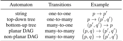
Finite automata generate strings by transitioning from state to state. Top-down tree automata gen-eralise string finite automata by transitioning from a state to an ordered sequence of states, generating trees top-down from root to leaves; while bottom-up tree automata transition from an ordered se-quence of states to a single state, generating trees bottom-up from leaves to root. The planar DAG automata ofKamimura and Slutzki(1981) gener-alise tree automata, transitioning from one ordered sequence of states to another ordered sequence of states (Section 4). Finally, the DAG automata ofQuernheim and Knight (2012) transition from multisetsof states to multisets of states, rather than from sequences to sequences, and this allows them to generate non-planar DAGs. We summarise the differences in Table1below.
Automaton Transitions Example
string one-to-one p→p0 top-down tree one-to-many p→(p0, q0)
bottom-up tree many-to-one (p0, q0)→p planar DAG many-to-many (p, q)→(p0, q0)
non-planar DAG many-to-many {p, q} → {p0, q0}
Table 1: The forms of transitions in different automata.
[image:2.595.309.525.490.562.2]b a
b
c b
a a
(iii) (ii)
(i)
q
q
p0
t2, t3
q
p
t2 t1
p
t4 b
a
b
c
d
(iv) q
p0 t4, t5 b a
b
c
d d e
(v)
p
p q
p q
p0 p0 p0
a
b
b
c
d d e
(vii) b
a
b
c
d
(vi)
p
p q
p q
p0 p0 p0
t4, t5 t4
from (iii)
[image:3.595.75.525.64.145.2]q p0
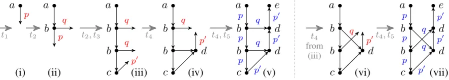
Figure 2: Two derivations using the automaton of Example1. Parts (i), (ii), and (iii) are common to both deriva-tions. Parts (iv) and (v) represent one completion, while (vi) and (vii) represent an alternative completion. Grey double edges denote derivation steps, labeled with the corresponding transition(s); red edge labels on partial graphs (i–iv) and (vi) denote frontier states; blue edge labels on complete graphs (v) and (vii) denote an accepting run.
q’s, and since multisets are unordered, it can also be written{q, p, q}or{q, q, p}. We write∅for a multiset containing no elements.
Definition 2. ADAG automatonis a tripleA = (Q,Σ, T) whereQis a finite set of states; Σis a finite set of node labels; and T is a finite set of transitions of the formα −→σ β whereσ ∈ Σis a node label,α ∈ M(Q) is the left-hand side, and β ∈M(Q)is the right-hand side.
Example 1. Let A = (Q,Σ, T) be a DAG au-tomaton whereQ={p, p0, q},Σ ={a, b, c, d, e} and the transitions inT are as follows:
∅−→ {p}a (t1)
{p}−→ {p, q}b (t2)
{p}−→ {pc 0} (t3)
{p0, q}−→ {pd 0} (t4)
{p0}−→ ∅e (t5)
2.1.1 Generating Single-rooted DAGs
A DAG automaton generates a graph from root to leaves. To illustrate this, we’ll focus on the case where a DAG is allowed to have only a single root, and return to the multi-rooted case in Section
3.1. To generate the root, the DAG automaton can choose any transition with∅on its left-hand side— these transitions behave like transitions from the start state in a finite automaton on strings, and always generate roots. In our example, the only available transition ist1, which generates a node
labeled awith a dangling outgoing edge in state p, as in Figure2(i). The set of all such dangling edges is thefrontierof a partially-generated DAG. While there are edges on the frontier, the DAG automation must choose and apply a transition whose left-hand side matches some subset of them. In our example, the automaton can choose eithert2ort3, each matching the availablepedge.
The edges associated with the matched states are attached to a new node with new outgoing frontier
edges specified by the transition, and the matched states are removed from the frontier. If our au-tomaton choosest2, it arrives at the configuration
in Figure 2(ii), with a new node labeled b, new edges on the frontier labeledpandq, and the in-coming p state forgotten. Once again, it must choose betweent2andt3—it cannot use theqstate
because that state can only be used byt4, which
also requires ap0 on the frontier. So each time it appliest2, the choice betweent2andt3repeats.
If the automaton applies t2 again and then t3,
as it has done in Figure 2(iii), it will face a new set of choices, betweent4 andt5. But notice that
choosingt5 will leave theq states stranded,
leav-ing a partially derived DAG. We consider a run of the automaton successful only when the frontier is empty, so this choice leads to a dead end.
If the automaton choosest4, it has an additional
choice: it can combinep0 witheitherof the avail-able q states. If it combines with the lowermost q, it arrives at the graph in Figure 2(iv), and it can then applyt4to consume the remainingq,
fol-lowed by t5, which has ∅ on its right-hand side.
Transitions to ∅ behave like transitions to a fi-nal state in a finite automaton, and generate leaf nodes, so we arrive at the complete graph in Fig-ure2(v). If thep0state in Figure2(iii) had instead combined with the upperq, a different DAG would result, as shown in Figure2(vi-vii).
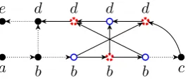
The DAGs in Figure 2(v) and Figure2(vii) are planar, which means they can be drawn without crossing edges.1 But this DAG automaton can also produce non-planar DAGs like the one in Fig-ure3. To see that it is non-planar, we firstcontract each dotted edge by removing it and fusing its end-points into a single node. This gives us theminor
1While the graph in Figure2(vii) is drawn with crossing
subgraphK3,3, and any graph with aK3,3 minor
is non-planar (Wagner,1937).
a b b b b c
[image:4.595.116.250.104.161.2]d d d d e
Figure 3: A non-planar graph that can be generated by the automaton of Example1. When the dotted edges are contracted, we obtain K3,3, the complete
(undi-rected) bipartite graph over two sets of three nodes. One set is denoted by hollow blue nodes ( ), the other by dotted red nodes ( ).
2.1.2 Recognising DAGs and DAG Languages
We define the language generated by a DAG au-tomaton in terms of recognition, which asks if an input DAG could have been generated by an input automaton. We recognise a DAG by finding a run of the automaton that could have generated it. To guess a run on a DAG, we guess a state for each of its edges, and then ask whether those states simu-late a valid sequence of transitions.
A run of a DAG automaton A = (Q,Σ, T) on a DAG G = (V, E,lab,src,tar) is a map-ping ρ : E → Q from edges of G to automa-ton statesQ. We extend ρto multisets by saying ρ({e1, . . . , en}) = {ρ(e1), . . . , ρ(en)}, and we
call a runacceptingif for allv∈V there is a
cor-responding transitionρ(IN(v))−−−→lab(v) ρ(OUT(v)) in T. DAG Gis recognised by automaton A if there is an accepting run ofAonG.
Example 2. The DAGs in Figure 2(v) and2(vii) are recognised by the automaton in Example 1. The only accepting run for each DAG is denoted by the blue edge labels.
The single-rooted languageLs(A) of a DAG automatonAis{G∈ G1
Σ |ArecognizesG}.
2.2 Probability and Weighted DAG Automata
Definition 3. Given a language L of DAGs, a
probability distribution over L is any function p:L→Rmeeting two requirements:
(R1) Every DAG must have a probability between 0 and 1, inclusive. Formally, we require that for allG∈L,p(G)∈[0,1].
(R2) The probabilities of all DAGs must sum to one. Formally, we requireP
G∈Lp(G) = 1.
R1 and R2 suffice to define a probability distri-bution, but in practice we need something stronger than R1: all DAGs must receive anon-zeroweight, since in practical applications, objects with proba-bility zero are effectively not in the language.
Definition 4. A probability distributionphasfull supportofLif and only if it meets condition R1’.
(R1’) Every DAG must have a probability greater than 0 and less than or equal to 1. Formally, we require that for allG∈L,p(G)∈(0,1].
While there are many ways to define a func-tion that meets requirements R1’ and R2, proba-bility distributions in natural language processing are widely defined in terms of weighted automata or grammars, so we adapt a common definition of weighted grammars (Booth and Thompson,1973) to DAG automata.
Definition 5. A weighted DAG automaton is a pair (A, w) where A = (Q,Σ, T) is a DAG au-tomaton andw:T →Ris a function that assigns real-valued weights to the transitions ofA.
Since weights are functions of transitions, we will write them on transitions following the node label and a slash (/). For example, ifp −→a q is a
transition and2is its weight, we writep−−→a/2 q.
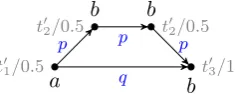
Example 3. Let (A, w) be a weighted DAG au-tomaton withA = (Q,Σ, T), whereQ ={p, q}, Σ = {a, b, c}, and the weighted transitions of T are as follows:
∅−−−→ {p, q}a/0.5 (t01)
{p}−−−→ {p}b/0.5 (t02)
{p, q}−−→ ∅c/1 (t03)
We use the weights on transitions to weight runs.
Definition 6. Given a weighted DAG automaton (A, w) and a DAGG = (V, E,lab,src,tar)with an accepting run ρ, we extend w to compute the
weight of the runw(ρ)by multiplying the weights of all of its transitions:
w(ρ) = Y
v∈V
w(ρ(IN(v))−−−→lab(v) ρ(OUT(v)))
Example 4. The DAG automaton of Example 3
t01/0.5
a
t02/0.5
b
t02/0.5
b
t03/1
b
p
q
[image:5.595.123.241.66.113.2]p p
Figure 4: A DAG generated by the automaton in Exam-ple3. Blue edge labels denote an accepting run; grey node labels denote weighted transitions used in the run.
LetRA(G)be the set of all accepting runs of a DAGGusing the automatonA. We extendw to calculate the weight of a DAGGas the sum of the weights of all the runs that produce it:
w(G) = X
ρ∈RA(G)
w(ρ).
While all weighted DAG automata assign real values to DAGs, not all weighted DAG automata define probability distributions. To do so, they must also satisfy requirements R1 and R2.
Definition 7. A weighted automaton(A, w)over languageL(A)isprobabilisticif and only if func-tionw:L(A)→Ris a probability distribution.
Example 5. Consider the weighted automaton in Example3. Every DAG generated by this automa-ton must uset01andt03exactly once, and can uset02 any number of times. If we let Gn be the DAG that uses t02 exactly n times, then the language L defined by this automaton is S
n∈NGn. Since
w(Gn) = w(t01)w(t02)nw(t03) and w(t01), w(t02)
andw(t03)are positive,wsatisfies R1 and:
X
G∈L
w(G) =
∞
X
n=0
w(Gn) =
∞
X
n=0
w(t01)w(t02)nw(t03)
=
∞
X
n=0
0.5n+1= 1
Thuswalso satisfies R2 and the weighted automa-ton in Example3is probabilistic.
Definition 8. A probabilistic automaton (A, w) over languageL(A)isprobabilistic with full sup-portif and only ifwhas full support ofL(A).
For every finite automaton over strings or trees, there is a weighting of its transitions that makes it probabilistic (Booth and Thompson,1973), and it is easy to show that it can be made probabilistic with full support. For example, string finite au-tomata have full support if for every state the sum of weights on its outgoing transitions is 1 and each
weight is greater than 0.2 But as we will show, this is not always possible for DAG automata.
3 Non-probabilistic DAG Automata
We will exhibit a DAG automaton that generates factorially many DAGs for a given number of nodes, and we will show that for any nontrivial assignment of weights, this factorial growth rate causes the weight of all DAGs to sum to infinity. Theorem 1. Let A be the automaton defined in Example1. There is nowthat makes(A, w) prob-abilistic with full support overLs(A).
Proof. In any run of the automaton, transitiont1
is applied exactly once to generate the single root, placing apon the frontier. This gives a choice be-tween t2 andt3. If the automaton chooses t2, it
keeps onepon the frontier and adds aq, and must then repeat the same choice. Suppose it chooses t2exactlyntimes in succession, and then chooses
t3. Then the frontier will containnedges in state
q and one in state p0. The only way to consume all of the frontier states is to apply transitiont4
ex-actlyntimes, consuming aqat each step, and then apply t5 to consumep0 and complete the
deriva-tion. Hence in any accepting run,t1, t3 andt5are
each applied once, andt2 andt4 are each applied
ntimes, for somen ≥ 0. Since transitions map uniquely to node labels, it follows that every DAG inLs(A)will have exactly one node each labeled a,c, ande; andnnodes each labeledbandd.
When the automaton appliest4for the first time,
it hasnchoices ofq states to consume, each dis-tinguished by its unique path from the root. The second application oft4hasn−1choices ofq, and
theith application oft4 hasn−(i−1)choices.
Therefore, there aren!different ways to consume theqstates, each producing a unique DAG.
Let f(n) be the weight of a run where t2 has
been appliedntimes, and to simplify our notation, letB = w(t1)w(t3)w(t5), andC =w(t2)w(t4).
Letc(n) be the number of unique runs wheret2
has been appliedntimes. By the above:
f(n) =w(t1)w(t2)nw(t3)w(t4)nw(t5) =BCn
c(n) =n!
Now we claim that any DAG inLs(A)has ex-actly one accepting run, because the mapping of
2Assuming no epsilon transitions, in our notation for DAG
node labels to transitions also uniquely determines the state of each edge in an accepting run. For ex-ample, a b node must result from a t2 transition
and a d node from a t4 transition, and since the
output states oft2and input states oft4share only
aq, any edge from abnode to adnode must be la-beledqin any accepting run. Now letG∈Ls(A) be a DAG with nnodes labeled b. Since G has only one accepting run, we have:
w(G) =f(n)
LetLnbe the set of all DAGs inLs(A)withn nodes labeledb. ThenLs(A) =S∞n=0Lnand:
X
G∈Ls(A)
w(G) =
∞
X
n=0
X
G∈Ln
w(G) =
∞
X
n=0
c(n)f(n)
=
∞
X
n=0
(n!) BCn
Hence for (A, w) to be probabilistic with full support, R1’ and R2 require us to choose B and C so that, respectively, BCn ∈ (0,1] for all n andP∞
n=0n!BCn = 1. Note that this does not
constrain the component weights ofB orC to be in(0,1]—they can be any real numbers. But since R1’ requires BCn to be positive for all n, both B andC must also be positive. If either were 0, then BCn would be 0 for n > 0; if either were negative, then BCn would be negative for some or all values ofn.
Now we show that any choice of positive C causesP
G∈Ls(A)w(G) to diverge. Given an
in-finite series of the formP∞
n=0an, the ratio test
(D’Alembert, 1768) considers the ratio between adjacent terms in the limit,limn→∞|a|na+1n||. If this
ratio is greater than 1, the series diverges; if less than 1 the series converges; if exactly 1 the test is inconclusive. In our case:
lim n→∞
|(n+ 1)!BCn+1|
|n!BCn| = limn→∞(n+ 1)|C|=∞.
Hence P
G∈Ls(A) diverges for any choice ofC,
equivalently for any choice of weights. So there is nowfor which(A, w)is probabilistic with full support overLs(A).
Note that any automaton recognising Ls(A) must accept factorially many DAGs in the number of nodes. Our proof implies that there isno proba-bilistic DAG automaton for languageLs(A), since
no matter how we design its transitions—each of which must be isomorphic to one inAapart from the identities of the states—the factorial will even-tually overwhelm the constant factor correspond-ing toCin our proof, no matter how small it is.
Theorem 1 does not rule out all probabilistic variants ofA. It requires R1’—if we only require the weaker R1, then a solution of B=1 and C=0 makes the automaton probabilistic. But this trivial distribution is not very useful: it assigns all of its mass to the singleton language{ a c e}. Theorem1also does not mean that it is impossi-ble to define a probability distribution overLs(A) with full support. If, for every DAG G with n nodes labeledb, we letp(G) = 2n+11 n!, then:
X
G∈Ls(A)
w(G) =
∞
X
n=0
1
2n+1n!n! = ∞
X
n=0
1 2n+1 = 1
But this distribution does not factor over transi-tions, so it cannot be used with the dynamic pro-gramming algorithms ofChiang et al.(2018).
A natural way to define distributions using a DAG automaton is to define two conditional prob-abilities: one over the choice of nodes to rewrite, given a frontier; and one over the choice of tran-sition, given the chosen nodes. The latter factors over transitions, but the former does not, so it also cannot use the algorithms ofChiang et al.(2018).3 Theorem 1 only applies to single-rooted, non-planar DAG automata of bounded degree. Next we ask whether it extends to other DAG automata, including those that recognise multi-rooted DAGs, DAGs of unbounded degree, and planar DAGs.
3.1 Multi-rooted DAGs
What happens when we consider DAG languages that allow multiple roots? In one reasonable inter-pretation of AMRbank, over three quarters of the DAGs have multiple roots (Kuhlmann and Oepen,
2016), so we want a model that permits this.4 Section2.1.1explained how a DAG automaton can be constrained to generate single-rooted lan-guages, by restricting start transitions (i.e. those
3In this model, the subproblems of a natural dynamic
pro-gram depend on the set of possible frontiers, rather than sub-sets of nodes as in the algorithms ofChiang et al.(2018). We do not know whether this could be made efficient.
4
with∅on the left-hand side) to a single use at the start of a derivation. To generate DAGs with mul-tiple roots, we simply allow start transitions to be applied at any time. We still require the result-ing DAGs to be connected. For an automatonA, we define its multi-rooted language Lm(A) as {G∈ G∗
Σ|ArecognisesG}.
Although one automaton can define both single-and multi-rooted DAG languages, these languages are incomparable.Drewes(2017) uses a construc-tion very similar to the one in Theorem1to show that single-rooted languages have very expressive path languages, which he argues are too expressive for modeling semantics.5 Since the constructions are so similar, it natural to wonder if the problem that single-rooted automata have with probabili-ties is related to their problem with expressivity, and whether it likewise disappears when we allow multiple roots. We now show that multi-rooted languages have the same problem with probabil-ity, because any multi-rooted language contains the single-rooted language as a sublanguage.
Corollary 1. Let Abe the automaton defined in Example1. There is nowthat makes(A, w) prob-abilistic with full support overLm(A).
Proof. By their definitions,Ls(A)⊂Lm(A), so:
X
G∈Lm(A)
w(G) =
X
G∈Ls(A)
w(G) + X
G∈Lm(A)\Ls(A)
w(G)
The first term is∞by Theorem1and the second is positive by R1’, so the sum diverges. Hence there is nowfor which(A, w)is probabilistic with full support overLm(A).
3.2 DAGs of Unbounded Degree
The maximum degree of any node in any DAG recognised by a DAG automaton is bounded by the maximum number of states in any transition, because any transition α −→σ β generates a node with|α|incoming edges and |β|outgoing edges. So, the families of DAG languages we have con-sidered all have bounded degree.
5
Thepath languageof a DAG is the set of strings that label a path from a root to a leaf, and the path language of a DAG language is the set of all such strings over all DAGs. For example, the path language of the DAG in Figure2(v) is
{abde, abbdde, abbcdde}. Berglund et al.(2017) show that path languages of multi-rooted DAG automata are regular, while those of single-rooted DAG automata characterised by a partially blind multi-counter automaton.
DAG languages with unbounded degree could be useful to model phenomena like coreference in meaning representations, and they have been stud-ied byQuernheim and Knight(2012) andChiang et al.(2018). These families generalise and strictly contain the family of bounded-degree DAG lan-guages, so they too, include DAG automata that cannot be made probabilistic.
3.3 Implications for semantic DAGs
We introduced DAG automata as a tool for model-ing the meanmodel-ing of natural language, but the DAG automaton in Theorem 1is very artificial, so it’s natural to ask whether it has any real relevance to natural language. We will argue informally that this example illustrates a pervasive problem with DAG automata—specifically, we conjecture that the factorial growth we observe in Theorem1
arises under very mild conditions that arise natu-rally in models of AMR.
Consider object control in a sentence like “I help Ruby help you” and its AMR in Figure5.
help
I
help
Ruby you
ARG1 ARG0
ARG2
[image:7.595.361.474.374.444.2]ARG0 ARG2
Figure 5: The AMR for “I help Ruby help you”.
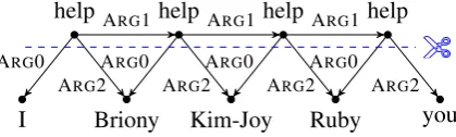
We can extend the control structure unbound-edly with additional helpers, as in “I help Briony help Kim-Joy help Ruby help you”, and this leads to unboundedly long repetitive graphs like the one in Figure6. These graphs can be cut to separate the sequence of “help” predicates from their argu-ments, as illustrated by the dashed blue line.
I help
Briony help
Kim-Joy help
Ruby help
you ARG1
ARG0 ARG2
ARG1
ARG0 ARG2
ARG1
ARG0 ARG2
ARG0 ARG2
Figure 6: The AMR for “I help Briony help Kim-Joy help Ruby help you” shown with a cut.
[image:7.595.313.523.596.659.2]could have been the frontier of a partially-derived graph. What if the number of edges in a cut—or cut-width—can be unbounded, as in the language of AMR graphs that model object control?
Since a DAG automaton can have only a finite number of states, there is some state that can occur unboundedly many times in a graph cut. All edges in a cut with this state can be rewired by permuting their target nodes, and the resulting graph will still be recognised by the automaton, since the rewiring would not change the multiset of states into or out of any node. If each possible rewiring results in a unique graph then the number of recognised graphs will be factorial in the number of source nodes for these edges, and the argument of Theo-rem1can be generalised to show that no weight-ing of any DAG automaton over the graph lan-guage makes it probabilistic with full support. For example, in the graph above, all possible rewirings of the ARG2 edges result in a unique graph.6 Al-though edge labels are not states, their translation into node labels implies that they can only be asso-ciated to a finite number of transitions, hence to a finite number of states in any corresponding DAG automaton. A full investigation of conditions un-der which Theorem 1 generalises is beyond the scope of this paper.
Conjecture 1. Under mild conditions, if language L(A)of a DAG automatonAhas unbounded cut-width, there is nowthat makes(A, w) probabilis-tic with full support.
4 Planar DAG Automata
The fundamental problem with trying to assign probabilities to non-planar DAG automata is the factorial growth in the number of DAGs with re-spect to the number of nodes. Does this problem occur in planar DAG automata?
Planar DAG automata are similar to the DAG automata of Section2but with an important differ-ence: they transition betweenordered sequences of states rather than unordered multisets of states. We write these sequences in parentheses, and their order matters: (p, q)differs from(q, p). We write for the empty sequence. When a planar DAG automaton generates DAGs, it keeps a strict order over the set of frontier states at all times. A transi-tion whose left-hand side is(p, q)can only be ap-plied to adjacent statespandqin the frontier, with
6This is also a problem linguistically, since many of the
rewired graphs no longer model object control.
pprecedingq. The matched states are replaced in the frontier by the sequence of states in the transi-tion’s right-hand side, maintaining order.
Example 6. Consider a planar DAG automaton with the following transitions:
−→a (p) (t001)
(p)−→b (p, q) (t002)
(p)−→c (p0) (t003)
(p0, q)−→d (p0) (t004)
(p0)−→e (t005)
In the non-planar case,napplications oft2 can
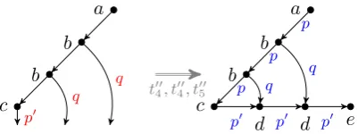
generate n!unique DAGs, but n applications of the corresponding transition t002 in this automaton can only generate one DAG. To see this, consider the partially derived DAG on the left of Figure7, with its frontier drawn in order from left to right. Thep0state can only combine with theqstate im-mediately to its right, and since dead-ends are not allowed, the only possible choice is to apply t004 twice followed byt005, so the DAG on the right is the only possible completion of the derivation.
a
b
b
c
d d e
b b
a
c
p
p
p
p0 p0 p0
q q t004, t
00
4, t
00
5
p0
[image:8.595.317.518.368.443.2]q q
Figure 7: A partial derivation using the planar DAG automaton of Example6 (left; red edge labels denote frontier states) and its only possible completion (right; blue edge labels denote an accepting run).
This automaton is probabilistic whenw(t001) = w(t002) = 1/2,w(t00
3) = w(t004) = w(t005) = 1, and
indeed the argument in Theorem1does not apply to planar automata since the number of applicable transitions is linear in the size of the frontier. But planar DAG automata have other problems that make them unsuitable for modeling AMR.
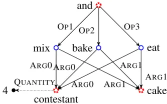
The first problem is that there are natural lan-guage constructions that naturally produce non-planar DAGs in AMR. For example, consider the sentence “Four contestants mixed, baked and ate cake.” Its AMR, shown in Figure 8, is not pla-nar because it has a K3,3 minor, and it is easy
to see from this example that any coordination of three predicates sharing two arguments produces this structure. In the first release of AMR, 117 out of 12844 DAGs are non-planar.
au-and
bake
mix eat
contestant
4 cake
OP1 O
P2 OP3
ARG0
ARG1 ARG0 ARG1
[image:9.595.96.263.65.169.2]ARG0 ARG1 QUANTITY
Figure 8: An AMR for the sentence “Four contestants mixed, baked and ate a cake”. As in Figure3, contract-ing the dotted edge yields aK3,3 minor, with one set
denoted by hollow blue nodes ( ), the other by dotted red nodes ( ).
tomata model Type-0 string derivations by design (Kamimura and Slutzki, 1981). This seems more expressive than needed to model natural language and means that many important decision problems are undecidable—for example, emptiness, which is decidable in polynomial time for non-planar DAG automata (Chiang et al.,2018).
5 Conclusions
Table2 summarises the properties of several dif-ferent variants of DAG automata. It has been ar-gued that all of these properties are desirable for probabilistic models of meaning representations (Drewes, 2017). Since none of the variants sup-ports all properties, this suggests that no variant of the DAG automaton is a good candidate for mod-eling meaning representations. We believe other formalisms may be more suitable, including sev-eral subfamilies of hyperedge replacement gram-mars (Drewes et al.,1997) that have recently been proposed (Bj¨orklund et al., 2016;Matheja et al.,
2015;Gilroy et al.,2017).
non-planar planar bounded degree yes no yes
roots 1 1+ 1 1+ 1
probabilistic no no no no ? decidable yes yes yes yes no regular paths no yes no yes no
Table 2: DAG automata variants and their properties.
Acknowledgements
This work was supported in part by the EP-SRC Centre for Doctoral Training in Data Sci-ence, funded by the UK Engineering and Physical
Sciences Research Council (grant EP/L016427/1) and the University of Edinburgh. We thank Esma Balkir, Nikolay Bogoychev, Shay Co-hen, Marco Damonte, Federico Fancellu, Joana Ribeiro, Nathan Schneider, Miloˇs Stanojevi´c, Ida Szubert, Clara Vania, and the anonymous review-ers for helpful discussion of this work and com-ments on previous drafts of the paper.
References
Laura Banarescu, Claire Bonial, Shu Cai, Madalina Georgescu, Kira Griffitt, Ulf Hermjakob, Kevin Knight, Philipp Koehn, Martha Palmer, and Nathan Schneider. 2013. Abstract meaning representation for sembanking. InProceedings of the 7th Linguis-tic Annotation Workshop and Interoperability with Discourse, pages 178–186, Sofia, Bulgaria.
Martin Berglund, Henrik Bj¨orklund, and Frank Drewes. 2017. Single-rooted dags in regular dag languages: Parikh image and path languages. In Proceedings of the 13th International Workshop on Tree Adjoining Grammars and Related Formalisms, pages 94–101, Ume˚a, Sweden.
Henrik Bj¨orklund, Frank Drewes, and Petter Ericson. 2016. Between a rock and a hard place - uniform parsing for hyperedge replacement DAG grammars. In Language and Automata Theory and Applica-tions - 10th International Conference, LATA 2016, Prague, Czech Republic, March 14-18, 2016, Pro-ceedings, pages 521–532.
Johannes Blum and Frank Drewes. 2016. Properties of regular DAG languages. In Language and Au-tomata Theory and Applications - 10th International Conference, LATA 2016, Prague, Czech Republic, March 14-18, 2016, Proceedings, pages 427–438.
T.L. Booth and R.A. Thompson. 1973. Applying prob-ability measures to abstract languages.IEEE Trans-actions on Computers, 22(5):442–450.
David Chiang, Jacob Andreas, Daniel Bauer, Karl Moritz Hermann, Bevan Jones, and Kevin Knight. 2013. Parsing graphs with hyperedge replacement grammars. InProceedings of the 51st Annual Meeting of the Association for Computa-tional Linguistics (Volume 1: Long Papers), pages 924–932, Sofia, Bulgaria.
David Chiang, Frank Drewes, Daniel Gildea, Adam Lopez, and Giorgio Satta. 2018. Weighted DAG au-tomata for semantic graphs. Computational linguis-tics, 44(1).
Jean D’Alembert. 1768.Opuscules, volume V.
[image:9.595.83.282.585.651.2]Frank Drewes, Hans-J¨org Kreowski, and Annegret Ha-bel. 1997. Hyperedge replacement graph grammars. In Grzegorz Rozenberg, editor,Handbook of Graph Grammars and Computing by Graph Transforma-tion, pages 95–162. World Scientific.
Jeffrey Flanigan, Chris Dyer, Noah A. Smith, and Jaime Carbonell. 2016. Generation from abstract meaning representation using tree transducers. In Proc. of NAACL-HLT, pages 731–739.
Sorcha Gilroy, Adam Lopez, Sebastian Maneth, and Pi-jus Simonaitis. 2017. (Re)introducing regular graph languages. InProceedings of the 15th Meeting on the Mathematics of Language (MoL 15), pages 100– 113.
Tsutomu Kamimura and Giora Slutzki. 1981. Parallel and two-way automata on directed ordered acyclic graphs.Information and Control, 49(1):10–51.
Marco Kuhlmann and Stephan Oepen. 2016. Squibs: Towards a catalogue of linguistic graph banks. Com-putational Linguistics, 42(4):819–827.
Christoph Matheja, Christina Jansen, and Thomas Noll. 2015. Tree-Like Grammars and Separation Logic, pages 90–108. Springer International Pub-lishing, Cham.
Jonathan May, Kevin Knight, and Heiko Vogler. 2010. Efficient inference through cascades of weighted tree transducers. InProceedings of the 48th Annual Meeting of the Association for Computational Lin-guistics, ACL ’10, pages 1058–1066.
Mehryar Mohri, Fernando C. N. Pereira, and Michael Riley. 2008. Speech recognition with weighted finite-state transducers. In Larry Rabiner and Fred Juang, editors,Handbook on Speech Processing and Speech Communication, Part E: Speech recognition, pages 69–88. Springer.
Rik van Noord and Johan Bos. 2017. Neural semantic parsing by character-based translation: Experiments with abstract meaning representations. Computa-tional Linguistics in the Netherlands Journal, 7:93– 108.
Daniel Quernheim and Kevin Knight. 2012. Towards probabilistic acceptors and transducers for feature structures. InProceedings of the Sixth Workshop on Syntax, Semantics and Structure in Statistical Trans-lation, SSST-6 ’12, pages 76–85.