A methodology pruning the search space of six compiler transformations by addressing them together as one problem and by exploiting the hardware architecture details

(1)

A methodology pruning the search space of six compiler

transformations by addressing them together as one

problem and by exploiting the hardware architecture

details

KELEFOURAS, Vasileios <http://orcid.org/0000-0001-9591-913X>

Available from Sheffield Hallam University Research Archive (SHURA) at:

http://shura.shu.ac.uk/18351/

This document is the author deposited version. You are advised to consult the

publisher's version if you wish to cite from it.

Published version

KELEFOURAS, Vasileios (2017). A methodology pruning the search space of six

compiler transformations by addressing them together as one problem and by

exploiting the hardware architecture details. Computing, 99 (9), 865-888.

Copyright and re-use policy

See

http://shura.shu.ac.uk/information.html

(2)

Noname manuscript No.

(will be inserted by the editor)

A methodology pruning the search space of six

compiler transformations by addressing them

together as one problem and by exploiting the

hardware architecture details

Vasilios Kelefouras

the date of receipt and acceptance should be inserted later

Abstract Today’s compilers have a plethora of optimizations-transformations to choose from, and the correct choice, order as well parameters of transfor-mations have a significant/large impact on performance; choosing the correct order and parameters of optimizations has been a long standing problem in compilation research, which until now remains unsolved; the separate sub-problems optimization gives a different schedule/binary for each sub-problem and these schedules cannot coexist, as by refining one degrades the other. Re-searchers try to solve this problem by using iterative compilation techniques but the search space is so big that it cannot be searched even by using modern supercomputers. Moreover, compiler transformations do not take into account the hardware architecture details and data reuse in an efficient way.

In this paper, a new iterative compilation methodology is presented which reduces the search space of six compiler transformations by addressing the above problems; the search space is reduced by many orders of magnitude and thus an efficient solution is now capable to be found. The transformations are the following: loop tiling (including the number of the levels of tiling), loop unroll, register allocation, scalar replacement, loop interchange and data array layouts. The search space is reduced a) by addressing the aforementioned transformations together as one problem and not separately, b) by taking into account the custom hardware architecture details (e.g., cache size and associativity) and algorithm characteristics (e.g., data reuse).

The proposed methodology has been evaluated over iterative compilation and gcc/icc compilers, on both embedded and general purpose processors; it achieves significant performance gains at many orders of magnitude lower compilation time.

Keywords loop unroll, loop tiling, scalar replacement, register allocation, data reuse, cache, loop transformations, iterative compilation

Vasilios Kelefouras University of Patras

(3)

1 Introduction

Choosing the correct order and parameters of optimizations has long been known to be an open problem in compilation research for decades. Compiler writers typically use a combination of experience and insight to construct the sequence of optimizations found in compilers. The optimum sequence of opti-mization phases for a specific code, normally is not efficient for another. This is because the back end compiler phases (e.g., loop tiling, register allocation) and the scheduling sub-problems depend on each other; these dependencies require that all phases should be optimized together as one problem and not separately.

Towards the above problem, many iterative compilation techniques have been proposed; iterative compilation outperforms the most aggressive compi-lation settings of commercial compilers. In iterative compicompi-lation, a number of different versions of the program is generated-executed by applying a set of compiler transformations, at all different combinations/sequences. Researchers and current compilers apply i) iterative compilation techniques [1] [2] [3] [4], ii) both iterative compilation and machine learning compilation techniques (to decrease search space and thus compilation time) [5] [6] [7] [8] [9] [10], iii) both iterative compilation and genetic algorithms (decrease the search space) [11], [12], [13], [14], [15], [16], [4], iv) compiler transformations by using heuris-tics and empirical methods [17], v) both iterative compilation and statistical techniques [18], vi) exhaustive search [15]. These approaches require very large compilation times which limit their practical use. This has led compiler researchers use exploration prediction models focusing on beneficial areas of optimization search space [19], [20], [21], [22].

The problem is that iterative compilation requires extremely long compila-tion times, even by using machine learning compilacompila-tion techniques or genetic algorithms to decrease the search space; thus, iterative compilation cannot include all existing transformations and their parameters, e.g., unroll factor values and tile sizes, because in this case compilation will last for many many years. As a consequence, a very large number of solutions is not tested.

In contrast to all the above, the proposed methodology uses a different iterative compilation approach. Instead of applying exploration and predic-tion methods, it fully exploits the hardware (HW) architecture details, e.g., cache size and associativity, and the custom software (SW) characteristics, e.g., subscript equations (constraint propagation to the HW and SW param-eters); in this way, the search space is decreased theoretically by many orders of magnitude and thus an efficient schedule is now capable to be found, e.g., given the cache architecture details, the number of different tile sizes tested is decreased. In Subsect.4, I show that if the transformations addressed in this paper (including almost all different transformation parameters) are included to iterative compilation, the compilation time lasts from 109

(4)

The major contributions of this paper are the following. First, loop un-roll, register allocation and scalar replacement are addressed together as one problem and not separately, by taking into account data reuse and RF size (Subsection 3.1). Second, loop tiling and data array layouts are addressed to-gether as one problem, by taking into account cache size and associativity and data reuse (Subsection 3.2). Third, according to the two major contributions given above, the search space is reduced by many orders of magnitude and thus an efficient solution is now capable to be found.

The experimental results have taken by using PowerPC-440 and Intel Xeon Quad Core E3-1240 v3 embedded and general purpose processors, respectively. The proposed methodology has been evaluated for seven well-known data in-tensive algorithms over iterative compilation and gcc / Intel icc compilers (speedup values from 1.4 up to 3.3); the evaluation refers to both compilation time and performance.

The remainder of this paper is organized as follows. In Section 2, the re-lated work is given. The proposed methodology is given in Section 3 while experimental results are given in Section 4. Finally, Section 5 is dedicated to conclusions.

2 Related Work

Normally, iterative compilation methods include transformations with low compilation time such as common subexpression elimination, unreachable code elimination, branch chaining and not compile time expensive transformations such as loop tiling and loop unroll. Iterative compilation techniques either do not use loop tiling and loop unroll transformations at all, or they use them only for specific tile sizes, levels of tiling and unroll factor values [23] [24] [25]. In [23], one level of tiling is used with tile sizes from 1 up to 100 and unroll factor values from 1 up to 20 (innermost iterator only). In [24], multiple levels of tiling are applied but with fixed tile sizes. In [26], all tile sizes are considered but each loop is optimized in isolation; loop unroll is applied in isolation also. In [25], loop tiling is applied with fixed tile sizes. In [27] and [28], only loop unroll transformation is applied.

Regarding genetic algorithms, [11], [12], [13], [14], [15], [16], [4] show that selecting a better sequence of optimizations significantly improves execution time. In [12] a genetic algorithm is used to find optimization sequences re-ducing code size. In [11], a large experimental study of the search space of the compilation sequences is made. They examine the structure of the search space, in particular the distribution of local minima relative to the global min-ima and devise new search based algorithms that outperform generic search techniques. In [29] they use machine learning on a training phase to predict good polyhedral optimizations.

(5)

Moreover, they require a very large compilation time and they are difficult to implement.

[15] first reduces the search space by avoiding unnecessary executions and then modifies the search space so fewer generations are required. In [30] they suppose that some compiler phases may not interact with each other and thus, they are removed from the phase order search space (they apply them implicitly after every relevant phase).

[31] uses an artificial neural network to predict the best transformation (from a given set) that should be applied based on the characteristics of the code. Once the best transformation has been found, the procedure is repeated to find the second best transformation etc. In [32] prediction models are given to predict the set of optimizations that should be turned on. [20] address the problem of predicting good compiler optimizations by using performance counters to automatically generate compiler heuristics.

An innovative approach to iterative compilation was proposed by [33] where they used performance counters to propose new optimization sequences. The proposed sequences were evaluated and the performance counters are measured to choose the new optimizations to try. In [29], they formulate the selection of the best transformation sequence as a learning problem, and they use off-line training to build predictors that compute the best sequence of polyhedral optimizations to apply.

In contrast to all the above works, the proposed methodology methodol-ogy uses a different approach. Instead of applying exploration and prediction methods, the search space is decreased by fully utilizing the HW architecture details and the SW characteristics.

As far as register the allocation problem is concerned, many methodologies exist such as [34] [35] [36] [37] [38] [39] [40]. In [34] - [38], data reuse is not taken into account. In [39] and [40], data reuse is taken into account either by greedily assigning the available registers to the data array references or by applying loop unroll transformation to expose reuse and opportunities for max-imizing parallelism. In [41], a survey on combinatorial register allocation and instruction scheduling is given. Finally, regarding data cache miss elimination methods, much research has been done in [42] [43] [44] [45] [46] [47] [48].

3 Proposed Methodology

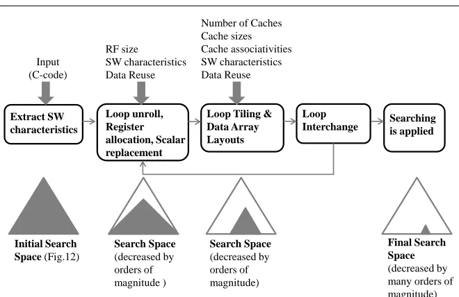
The proposed methodology takes the target C-code and HW architecture de-tails as input and automatically generates only the efficient schedules, while the inefficient ones are being discarded, decreasing the search space by many orders of magnitude, e.g., all the schedules using a larger number of registers than the available are discarded. Then, searching only among a specific set of efficient schedules is applied and an efficient schedule can be found fast.

(6)

1. Loop tiling to all the iterators (tiling for L1 cache )

 all different tile sizes are included 2. Loop tiling to all the iterators (tiling for L2

cache )

 all different tile sizes are included Search Space

The search space includes all these transformations at all different orderings (The number of combinations is up to 7 ! = 5040) 3. Scalar replacement

4. Register allocation

5. Loop unroll to all the iterators

 all different unroll factor values are included 6. Different data array Layouts 7. Loop interchange

Fig. 1 Search space being addressed.

is applied to all the iterators. Also it includes register allocation, scalar re-placement, loop unroll to all the iterators, loop interchange, and different data array layouts. In Fig. 1, there are seven different problems/transformations and thus the search space consists up to 7! = 5040 transformation combinations. In Subsect.4, I show that if the transformations presented in Fig.1 (including almost all different transformation parameters) are included to iterative com-pilation, the search space is from 1017

up to 1029

schedules(for the given input sizes); given that 1sec = 3.17×10−8

years and supposing that compilation

time takes 1 sec, the compilation time is from 109

up to 1021

years. On the

other hand, the proposed methodology decreases the search space from 101

up to 105

schedules. In this way, the search space is now capable to be searched in a short amount of time.

Regarding target applications, this methodology optimizes loop kernels; as it is well known, 90% of the execution time of a computer program is spent ex-ecuting 10% of the code (also known as the 90/10 law) [49]. The methodology is applied to both perfectly and imperfectly nested loops, where all the array subscripts are linear equations of the iterators (which in most cases do); an array subscript is another way to describe an array index (multidimensional arrays use one subscript for each dimension). This methodology can also be applied to C code containing SSE/AVX instructions (SIMD). For the reminder of this paper, I refer to architectures having separate L1 data and instruction cache (vast majority of architectures). In this case, the program code always fits in L1 instruction cache since I refer to loop kernels only, whose code size is small; thus, upper level unified/shared caches, if exist, contain only data. On the other hand, if a unified L1 cache exists, memory management becomes very complicated.

[image:6.595.74.400.78.246.2]

(7)

Extract SW characteristics

Loop unroll, Register allocation, Scalar replacement

Loop Tiling & Data Array Layouts

Loop

Interchange Searching _{is applied}

Input (C-code)

RF size

SW characteristics Data Reuse

Number of Caches Cache sizes Cache associativities SW characteristics Data Reuse

Initial Search Space (Fig.12)

Final Search Space

(decreased by many orders of magnitude)

Search Space

(decreased by orders of magnitude )

Search Space

(decreased by orders of magnitude)

Fig. 2 Flow graph of the proposed methodology

to apply the aforementioned transformations in an efficient way. One math-ematical equation is created for each array’s subscript in order to find the corresponding memory access pattern, e.g., (A[2∗i+j]) and (B[i, j]) give (2∗i+j=c1) and (i=c21 andj=c22), respectively, where (c1, c21, c22) are constant numbers and their range is computed according to the iterator bound values. Each equation defines the memory access pattern of the specific array reference; data reuse is found by these equations (data reuse occurs when a specific memory location is accessed more than once).

Regarding 2-d arrays, two equations are created and not one because the data array layout is not fixed, e.g., regardingB[i, j] reference, if (N∗i+j=c)

(whereN is the number of the array columns) is taken instead of (i=c1) and

(j=c2), then row-wise layout is taken which may not be efficient.

Definition 1 Subscript equations which have more than one solution for at least one constant value, are named type2 equations. All others, are named type1 equations, e.g., (2∗i+j =c1) is a type2 equation, while (i=c21 and

j=c22) is a type1 equation.

Arrays with type2 subscript equations are accessed more than once from memory (data reuse), e.g., (2i+j = 7) holds for several iteration vectors; on the other hand, equations of type1 fetch their elements only once; in [50], I give a new compiler transformation that fully exploits data reuse of type2 equations. However, both type1 and type2 arrays may be accessed more than once in the case that the loop kernel contains at least one iterator that does not exist in the subscript equation, e.g., consider a loop kernel containingk, i, j

[image:7.595.76.406.76.290.2]

(8)

Definition 2 The subscript equations which are not given by a compile time known expression (e.g., they depend on the input data), are further classified into type3 equations. Data reuse of type3 arrays cannot be exploited, as the arrays elements are not accessed according to a mathematical formula.

After the SW characteristics have been extracted, I apply loop unroll, reg-ister allocation and scalar replacement, in a novel way, by taking into account the subscript equations, data reuse and RF size (Subsection 3.1). I generate extra mathematical inequalities that give all the efficient RF tile sizes and shapes, according to the number of the available registers. All the schedules using a different number of registers than those the proposed inequalities give are not considered, decreasing the search space. Moreover, one level of tiling is applied for each cache memory (if needed), in a novel way, by taking into ac-count the cache size and associativity, the data array layouts and the subscript equations (Subsection 3.2). One inequality is created for each cache memory; these inequalities contain all the efficient tile sizes and shapes, according to the cache architecture details. All tile sizes and shapes and array layouts different than those the proposed inequalities give are not considered decreasing the search space.

It is important to say that partitioning the arrays into tiles according to the cache size only is not enough because tiles may conflict with each other due to the cache modulo effect. Given that all the tiles must remain in cache, a) all the tile elements have to be written in consecutive main memory locations and therefore in consecutive cache locations (otherwise, the data array layout is changed), and b) different array tiles have to be loaded in different cache ways in order not to conflict with each other. All the schedules with different tile sizes than those the proposed inequalities give are not considered, decreasing the exploration space even more.

In contrast to iterative compilation methods, the number of levels of tiling is not one, but it depends on the number of the memories. For a two level cache architecture, loop tiling is applied for a) L1, b) L2, c) L1 and L2, and d) none. The number of levels of tiling is found by testing as the data reuse advantage can be overlapped by the extra inserted instructions; although the number of data accesses is decreased (by applying loop tiling), the number of addressing instructions (and in several cases the number of load/store instructions) is increased.

When the above procedure has ended, all the efficient transformation pa-rameters have been found (according to the Subsections 3.1 and 3.2) and all the inefficient parameters have been discarded reducing the search space by many orders of magnitude. Then, all the remaining schedules are automat-ically transformed into C-code; the C-codes are generated by applying the aforementioned transformations with the parameters found in Subsections 3.1 and 3.2. Afterwards, all the C-codes are compiled by the target architecture compiler and all the binaries run to the target platform to find the fastest.

(9)

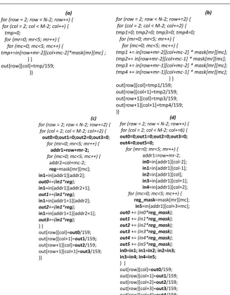
(b)

for (row = 2; row < N-2; row+=2) { for (col = 2; col < M-2; col+=2) { tmp1=0; tmp2=0; tmp3=0; tmp4=0;

for (mr=0; mr<5; mr++) { for (mc=0; mc<5; mc++) {

tmp1 += in[row+mr-2][col+mc-2] * mask[mr][mc]; tmp2+= in[row+mr-2][col+mc-1] * mask[mr][mc]; tmp3 += in[row+mr-1][col+mc-2] * mask[mr][mc]; tmp4 += in[row+mr-1][col+mc-1] * mask[mr][mc];

} } out[row][col]=tmp1/159; out[row][col+1]=tmp2/159; out[row+1][col]=tmp3/159; out[row+1][col+1]=tmp4/159; }} (a)

for (row = 2; row < N-2; row++) { for (col = 2; col < M-2; col++) {

tmp=0;

for (mr=0; mr<5; mr++) { for (mc=0; mc<5; mc++) {

tmp+=in[row+mr-2][col+mc-2]*mask[mr][mc] ; } }

out[row][col]=tmp/159; }}

(c)

for (row = 2; row < N-2; row+=2) { for (col = 2; col < M-2; col+=2) {

out0=0;out1=0;out2=0;out3=0; for (mr=0; mr<5; mr++) {

addr1=row+mr-2;

for (mc=0; mc<5; mc++) { addr2=col+mc-2;

reg=mask[mr][mc];

in1=in[addr1][addr2];

out0+=(in1*reg);

in1=in[addr1][addr2+1];

out1+=(in1*reg);

in1=in[addr1+1][addr2];

out2+=(in1*reg);

in1=in[addr1+1][addr2+1];

out3+=(in1*reg); } }

out[row][col]=out0/159; out[row][col+1]=out1/159;

out[row+1][col]=out2/159; out[row+1][col+1]=out3/159; }}

(d)

for (row = 2; row < N-2; row++) { for (col = 2; col < M-2; col+=6) {

out0=0;out1=0;out2=0;out3=0; out4=0;out5=0;

for (mr=0; mr<5; mr++) { addr1=row+mr-2; in0=in[addr1][col-2]; in1=in[addr1][col-1]; in2=in[addr1][col]; in3=in[addr1][col+1]; in4=in[addr1][col+2]; for (mc=0; mc<5; mc++) {

reg_mask=mask[mr][mc];

in5=in[addr1][col+3+mc];

out0+= (in0*reg_mask);

out2 += (in2*reg_mask);

in0=in1; in1=in2; in2=in3; in3=in4; in4=in5;

} }

out[row][col]=out0/159; out[row][col+1]=out1/159; out[row][col+2]=out2/159; out[row][col+3]=out3/159; out[row][col+4]=out4/159; out[row][col+5]=out5/159; } }

Fig. 3 An example, Gaussian Blur algorithm

3.1 Loop unroll, scalar replacement, register allocation

[image:9.595.78.406.75.496.2]

(10)

body exposes data reuse (In Fig. 3-(b), loop unroll is applied to the first two iterators with unroll factor values equal to 2, while in Fig. 3-(c) the common array references are replaced by variables). However, the number of common array references exposed depends on the iterators that loop unroll is being applied to and on the loop unroll factor values. Unrolling the correct iterator exposes data reuse; on the other hand, in Rule2, I show that data reuse cannot be exposed by applying loop unroll to the innermost iterator. Regarding the loop unroll factor values, they depend on the RF size; the larger the loop unroll factor value, the larger the number of the registers needed. Moreover, the unroll factor values and the number of the variables/registers used, depend on data reuse, as it is efficient to use more variables/registers for the array references that achieve data reuse and less for the references that do not. Thus, the above problems are strongly interdependent and it is not efficient to be addressed separately.

The number of assigned variables/registers is given by the following in-equality. I generate mathematical inequalities that give all the efficient RF tile sizes and shapes, according to the number of the available registers. All the schedules with different number of registers than those the proposed inequali-ties give are not considered, decreasing the search space. In contrast to all the related works, the search space is decreased not by applying exploration and prediction methods but by fully utilizing the RF size.

The register file inequality is given by:

0.7×RF ≤Iterators+Scalar+Extra+Array1+Array2+...+Arrayn≤RF (1)

where RF is the number of available registers, Scalar is the number of

scalar variables,Extra is the number of extra registers needed, i.e., registers

for intermediate results andIterators is the number of the different iterator

references exist in the innermost loop body, e.g., in Fig. 3-(b), (Iterators= 4), these are (row, mr, col, mc). Arrayi is the number of the variables/registers allocated for the i-th array.

Rule 1 TheArrayi values are found by ineq. 2 and Rules 5. I give Rules

2-5 to allocate registers according to the data reuse.

Arrayi=it′1×it′2×...×it′n (2)

where the integer it′

i are the unroll factor values of the iterators exist in the array’s subscript; e.g. forB(i, j) andC(i, i),ArrayB=i′×j′(rectangular tile) andArrayC=i′ (diagonal line tile) respectively, where i′ andj′ are the unroll factors ofi,j iterators.

Each subscript equation contributes to the creation of ineq.( 1), i.e.,

equa-tion i gives Arrayi and specifies its expression. To my knowledge, no other

work uses a similar approach.

(11)

into binary code), the target compiler may not allocate the exact number

of desirable variables into registers. Moreover, the 0.7 value has been found

experimentally. The number ofScalarandExtraregisters are found after the

allocation of the array elements into variables/registers, because they depend on the unroll factor values and on the number of iterators being unrolled. The

Extravalue depends on the target compiler and thus it is found approximately; the bounds of the RF inequality are not tight for this reason too. The goal is to store all the inner loop reused array elements and scalar variables into registers minimizing the number of register spills.

Rules 2- 5 modify eq. 2 according to the data reuse. The array references that do not achieve data reuse do not use more than one register; on the other hand, the array references that achieve data reuse, use as many registers as possible according to the number of the available registers, e.g., in Fig. 3-(c) only one register is used for (in) and four for (out) array. To my knowledge, no other work takes into account data reuse in this way.

Rule 2 The innermost iterator is never unrolled because data reuse cannot be exposed; if iti is the innermost iterator, then it′i = 1.

Proof By unrolling the innermost iterator, the array references-equations which contain it, will change their values in each iteration; this means that i) a differ-ent elemdiffer-ent is accessed in each iteration and thus a huge number of differdiffer-ent registers is needed for these arrays, ii) all these registers are not reused (a dif-ferent element is accessed in each iteration). Thus, by unrolling the innermost iterator, more registers are needed which do not achieve data reuse; this leads to low RF utilization.

Rule 3 The type1 array references which contain all the loop kernel itera-tors, do not achieve data reuse (each element is accessed once); thus only one register is needed for these arrays, i.e., Arrayi = 1.

Proof The subscript equations of these arrays change their values in each it-eration vector and thus a different element is fetched in each itit-eration.

Let me give an example Gaussian Blur (Fig. 3). Suppose that loop unroll is applied torow, coliterators with unroll factor value equal to 2 (Fig. 3-(b)). Then, all array references are replaced by variables/registers according to the

register file size and data reuse (Fig. 3-(c)). Array out needs row′_×_col′ ₌

4 registers (Fig. 3) while array mask needs mr′_×_mc′ _{= 1 register, where}

row′_{, col}′_{, mr}′_{, mc}′ _{are the} _{row, col, mr, mc} _{unroll factor values, respectively.}

Although inarray needs 4 registers according to ineq. 2, it achieves no data

reuse and thus only one register is used (Rule 3). The number of registers needed for each array is given by its subscript equation; these equations give

the data access patterns and data reuse. Regarding mask array, it is reused

four times. Regardingoutarray, all its four references exist in the loop body

remain unchanged as the mr, mcchange, achieving data reuse.inarray does

not achieve data reuse and thus only one register is used for all the four

(12)

i₀=2; j₀=2;

for (jj=0; jj<M; jj+=T1)

for (i=0; i<N; i+=i₀) {

for(j=jj; j<jj+T1; j+=j₀) {

r1=0;r2=0;r3=0;r4=0;

for (k=0; k<P; k++) {

r5=A[i][k]; r6=A[i+1][k];

r7=B[j][k]; r8=B[j+1][k];

r1+=r5*r7; r2+=r5*r8; r3+=r6*r7; r4+=r6*r8;

}

C[i][j]=r1;

C[i][j+1]=r2;

C[i+1][j]=r3;

C[i+1][j+1]=r4;

} }

for (ii=0; ii<60; ii+=10)

for (jj=0; jj<60; jj+=15)

for (kk=0; kk<60; kk+=4)

for (i=ii; i<ii+10; i+=2)

for (k=kk; k<kk+4; k+=4) {

regA1=A[i][k]; regA2=A[i][k+1]; regA3=A[i][k+2]; regA4=A[i][k+3]; regA5=A[i+1][k]; regA6=A[i+1][k+1]; regA7=A[i+1][k+2]; regA8=A[i+1][k+3];

for (j=jj; j<jj+15; j++) {

regC1=0;regC2=0; regB1=B[k][j]; regB2=B[k+1][j];

regB3=B[k+2][j]; regB4=B[k+3][j];

regC1+=regA1 * regB1; regC1+=regA2 * regB2; regC1+=regA3 * regB3; regC1+=regA4 * regB4; regC2+=regA5 * regB1; regC2+=regA6 * regB2; regC2+=regA7 * regB3; regC2+=regA8 * regB4;

C[i][j]+=regC1; C[i+1][j]+=regC2;}}

(b)

(a)

Fig. 4 An example, Matrix-Matrix Multiplication

reuse between consecutive iterations ofmc; in Fig. 3-(d) this type of data reuse (Rule 5) is fully exploited by insertingin1−in5 registers. It is important to say that both Fig. 3-(c) and Fig. 3-(d), achieve a much smaller number of L/S and addressing instructions.

Rule 4 If there is an array reference i) containing more than one iterator and one of them is the innermost one and ii) all ineq.( 1) iterators which do not exist in this array reference have unroll factor values equal to1, then only one register is needed for this array, i.e. Arrayi = 1. This gives more than one

register file inequalities (it is further explained in the following example).

Proof When Rule 4 holds, a different array’s element is fetched in each itera-tion vector, as the subscript equaitera-tion changes its value in each iteraitera-tion. Thus, no data reuse is achieved and only one register is used. On the contrary, if at least one iterator which do not exist in this array reference is unrolled,

com-mon array references occur inside the loop body (e.g.,regC1 is reused 3 times

in Fig. 4); data reuse is achieved in this case and thus an extra RF inequality is created.

Let me give another example (Fig. 4-(a)). The C array subscript containsi

andjiterators.jiterator is the innermost one and thus (i′_×_{1 = 2) registers are}

[image:12.595.82.401.75.356.2]

(13)

registers ifk′₆_{= 1 and 1 register otherwise (if}_k′ _{= 1 then the C array fetches a}

different element in each iteration vector and thus only one register is needed). Regarding array A, it needsi′_×_k′ _{registers while B array needs}_k′ _{registers, if} i′₆_{= 1 and 1 register otherwise. Note that if the i-loop is not unrolled (}_i′_{= 0),}

the B and C array elements are not reused and thus there is 1 register for C

and 1 for B (Rule 4). The innermost iterator (j) is not unrolled according to

Rule 2 (data reuse is decreased in this case).

Moreover, there are cases that data reuse utilization is more complicated as common array elements may be accessed not in each iteration, but in each

kiterations, wherek≥1, e.g., Fig. 3-(d). This holds only for type2 equations

(e.g. ai+bj+c) wherek =b/a is an integer (data reuse is achieved in each

k iterations). Data reuse is exploited only when k = 1 here (Rule 5) as for

largerkvalues, data reuse is low. For example, in Fig. 3, each time the mask

is shifted by one position to the right (mciterator), 20 elements of in array

are reused (reuse between consecutive iterations, i.e.,k= 1).

Rule 5 Arrays with type2 subscript equations which have equal coefficient ab-solute values (e.g. ai+bj+c, where a == ±b) fetch identical elements in consecutive iterations; data reuse is exploited by interchanging the registers values in each iteration. An extra RF inequality is produced in this case.

Proof The arrays of Rule 5 access their elements in patterns. As the innermost iterator changes its value, the elements are accessed in a pattern, i.e. A[p],

A[p+b],A[p+ 2×b] etc. When the outermost iterator changes its value, this pattern is repeated, shifted by one position to the right (A[p+b],A[p+ 2×b],

A[p+ 3×b] etc), reusing its elements. This holds for equations with more than two iterators too.

To exploit data reuse of Rule 5, all the array’s registers interchange their values in each iteration, e.g., in Fig. 3 - (d), the (in0, in1, in2, in3, in4, in5) variables interchange their values in each iteration.

To sum up, by applying the aforementioned transformations as above, the number of i) load/store instructions (or equivalent the number of L1 data cache accesses) and ii) addressing instructions, are decreased. The number of load/store instructions is decreased because the reused references are assigned into registers and they reused as many times as the number of available regis-ters indicate. The number of addressing instructions is decreased because the address computations are simplified.

(14)

accesses. Moreover, all the schedules that do not satisfy the proposed Rules, do not take into account data reuse and thus several/many registers are wasted leading to a larger number of data accesses.

3.2 Loop tiling and data array layouts

Loop tiling is one of the key loop transformations to speedup data dominant applications. When the accumulated size of the arrays is larger than the cache size, the arrays do not remain in cache and in most cases they are loaded and reloaded many times from the slow main memory, decreasing performance and increasing energy consumption. In order to decrease the number of data accesses, loop tiling is applied, i.e., arrays are partitioned into smaller ones (tiles) in order to remain in cache achieving data locality.

Loop tiling for cache, cache size and associativity, data reuse and data array layouts, strongly depend on each other and thus they are addressed to-gether, as one problem and not separately. The reason follows. Let me give an example, Matrix-Matrix Multiplication algorithm. Many research works as well ATLAS [51] (one of the state of the art high performance libraries) apply loop tiling by taking into account only the cache size, i.e., the accumulated size of three rectangular tiles (one of each matrix) must be smaller or equal to the cache size; however, the elements of these tiles are not written in consecu-tive main memory locations (the elements of each tile sub-row are written in different main memory locations) and thus they do not use consecutive data cache locations; this means that having a set-associative cache, they cannot simultaneously fit in data cache due to the cache modulo effect. Moreover, even if the tile elements are written in consecutive main memory locations (different data array layout), the three tiles cannot simultaneously fit in data cache if the cache is two-way associative or direct mapped [52], [53]. Thus, loop tiling is efficient only when cache size, cache associativity and data array layouts, are addressed together as one problem and not separately.

For a 2 levels of cache architecture, 1 level of tiling (either for L1 or L2 cache), 2 levels of tiling and no tiling solutions, are applied to all the solutions-schedules that have been produced so far. The optimum number of levels of tiling cannot easily be found since the data locality advantage may be lost by the required insertion of extra L/S and addressing instructions, which degrade performance. The separate memories optimization gives a different schedule for each memory and these schedules cannot coexist, as by refining one, degrading another, e.g., the schedule minimizing the number of L2 data cache accesses and the schedule minimizing the number of main memory accesses cannot coexist; thus, either a sub-optimum schedule for all memories or a (near)-optimum schedule only for one memory can be produced.

(15)

not enough because tiles may conflict with each other due to the cache modulo effect; to satisfy that tiles remain in cache, first all the tile elements are written in consecutive main memory locations (in order to be loaded in consecutive cache locations), second different array tiles are loaded in different cache ways in order not to conflict with each other and third LRU cache replacement policy is used. All tile sizes and shapes and array layouts different than these the proposed inequalities give are not considered decreasing the search space.

The L1 data cache inequality is given by:

assoc−v−(⌊assoc/4⌋)≤ ⌈ T ile1 L1/assoc

⌉+...+⌈ T ilen L1/assoc

⌉ ≤assoc−v (3)

whereL1is the L1 data cache size andassocis the data cache associativity

(for an 8-way associative data cache,assoc= 8).vvalue is zero when no type3

array exist and one if at least one type3 array exists (it is explained next,

Rule 6). (⌊assoc/4⌋) gives the number of cache ways that remain unused and

defines the lower bound of tile sizes.T ilei is the tile size of the ith array and it is given by

T ilei=T1′×T2′×T_n′ ×ElementSize (4)

where integerT′

i are the tile sizes of the iterators that exist in the array’s

subscript. ElementSize is the size of each array’s element in bytes, e.g., in

Fig. 4-(a),T ileA=ii′×kk′×4 = 10×4×4,T ileB =kk′×jj′×4 = 15×4×4 andT ileC =ii′×jj′×4 = 10×15×4, if A,B and C contain floating point values (4 bytes each).

Ineq. 3 satisfies that no cache way contains more than one array’s elements, minimizing the number of cache conflicts.a1 =⌈ T ile1

L1/assoc⌉value is an integer and gives the number ofL1data cache lines with identicalL1addresses used for

T ile1. An empty cache line is always granted for each different modulo (with respect to the size of the cache) of Tiles memory addresses. For the reminder

of this paper I will more freely say that I use a1 cache ways for T ile1, a2

cache ways for T ile2 etc (in other words Tiles are written in separate data

cache ways). In the case that T ilei

L1/assoc would be used instead of ⌈ T ilei L1/assoc⌉,

the number ofL1 misses will be much larger because Tiles’ cache lines would

conflict with each other.

Moreover, in order to the Tiles remain in cache, their elements have to be written in consecutive cache locations and thus to consecutive main memory locations; thus, the data array layouts are changed to tile-wise (if needed), i.e., all array elements are written to main memory in order. To my knowledge, no other work addresses loop tiling by taking into account cache size, cache associativity and the data array layouts for a wide range of algorithms and computer architectures.

(16)

main memory locations but the associativity value is large enough to prevent cache conflicts, the data array layout remains unchanged, e.g., consider a 2-d array of sizeN×N and a tile of size 4×T, where T≺N; if (assoc≥4) and ((T×ElementSize)≺CacheW aySize), no cache conflict occurs.

Regarding type3 arrays, loop tiling cannot be applied. These arrays contain subscript equations which are not given by a compile time known expression (they depend on the input data). These arrays cannot be partitioned into tiles as their elements are accessed in a ’random’ way; this leads to a large number of cache conflicts due to the cache modulo effect (especially for large arrays). To eliminate these conflicts, Rule 6 is introduced.

Rule 6 For all the type3 arrays, data cache size which equals to the size of one cache way is granted (v= 1). In other words, an empty cache line is granted for each different modulo (with respect to the size of the cache) of these arrays memory addresses.

The search space is decreased even more by computing the best nesting level values of the new tiling iterators.

Statement 1 The nesting level values of the tiling iterators (produced by ap-plying loop tiling) are found theoretically (no searching is applied). This means that loop interchange is not applied to the new tiling iterators.

The nesting level values of the new (tiling) iterators are computed. For each different schedule produced by ineq.( 3), I compute the total number of data accesses for all the different nesting level values and the best are selected.

The number of each array’s accesses is found by:

DataAccesses = n×T ile size in elements×N um of tiles, where n is the number of times each tile is fetched and equals to (q×r), where qis the number of iterations exist above the upper iterator of the array’s equation and

ris the number of iterations exist between the upper and the lower iterators

of the array’s equation.

Last but not least, the search space is decreased by orders of magnitude without pruning efficient schedules. Although it is impractical to run all dif-ferent schedules (their number is huge) to prove that they are less efficient, they all give a much larger number of memory accesses in the whole memory hierarchy. All schedules that do not belong to ineq. 3, either use only a small portion of cache or a larger than the available or tile sizes do not use consecu-tive main memory / cache locations and thus they cannot remain in cache; in the first case, tile sizes are small giving a large number of data accesses and addressing instructions while in the second case, tile sizes are large and tiles cannot remain in cache leading to a much larger number of memory accesses.

4 Experimental Results

(17)

Evaluation Platform). Regarding Intel processor, a performance comparison is made over gcc 4.8.4 and Intel icc 2015 compilers; optimization level -O3 was

used at all cases. The operating system used is Ubuntu 14.04.

The comparison is done for 7 well-known data dominant linear algebra, image processing and signal processing kernels (PolyBench/C benchmark suite version 3.2 [54]). These are: Matrix Multiplication (MMM),

Matrix-Vector Multiplication (MVM), Gaussian Blur (5×5 filter), Finite Impulse

Response filter (FIR), Sobel operator (Manhattan distance is used instead of Euclidean distance), Jacobi 9-point Stencil and Gaussian Elimination. All the C-codes are single threaded and thus they run on one core only.

First, an evaluation of compilation time / search space is made over iter-ative compilation (iteriter-ative compilation here includes all the transformations

shown in Fig.1.). To the best of my knowledge there is no iterative

compilation method including the optimizations presented in this paper with all their parameters; iterative compilation techniques either do not use the transformations presented in this paper at all, or they use some them to some extent [23] [24] [25], e.g., loop tiling is applied only for spe-cific tile sizes and levels of tiling and loop unroll is applied only for spespe-cific unroll factor values. Normally, iterative compilation methods include transfor-mations with low compilation time such as common subexpression elimination, unreachable code elimination, branch chaining and not compile time expen-sive transformations such as loop tiling; I show that if the transformations presented in Fig.1 (including almost all different transformation parameters) are included in iterative compilation, the search space is from 1017

up to 1029 schedules(for the given input sizes) (Table 1); given that 1sec= 3.17×10−8 years and supposing that compilation time takes 1 sec, the compilation time is from 109

up to 1021

years. On the other hand, the proposed methodology

decreases the search space from 101

up to 105

schedules.

The first column of Table 1 gives the overall size of the search space (Fig. 1); the values have been computed by the following equation:

Schedules= 7!×(U nrollF actorloops×loops! + +U nrollF actorloops_×_{T ile}₁loops_×₍₂_×_loops_)!_×₍₂_×_matrices_{) +} +U nrollF actorloops×T ile2loops×(2×loops)!×(2×matrices) + +U nrollF actorloops×T ile1loops×T ile2loops×(3×loops)!×(2×matrices))(5)

where T ile1 and T ile2 are the numbers of different tile sizes for each

it-erator for the L1 and L2, respectively and loops is the number of the loops.

U nrollF actor value is the number of different unroll factor values for each

iterator. Finally, matrices is the number of multidimensional arrays and

(18)

The second and the fourth columns of Table1 give the search space size of the transformations used in Subsection 3.1 and Subsection 3.2, respectively.

The second column values of Table 1 are given by (4!×U nrollF actorloops_×

loops!). The fourth column values are obtained by (4!×T ile1loops_×_{T ile}₂loops_× (2×loops)!×(2×matrices)). The other column values have been obtained experimentally. The search space of MMM is the biggest as it contains 3 large loops to which loop tiling has applied. On the other hand, the smallest search space is that of MVM as it contains only two loops and a small input size.

For a fair comparison to be made, (U nrollF actor= 32), since the number

of the registers is limited. Moreover, the different tile sizes used here are the

following: for MMMT ile1 = 500 andT ile2 = 250, for Gaussian Blur, Sobel

and Jacobi stencil T ile1 = 600 and T ile2 = 300, for MVM T ile1 = 2100

and T ile2 = 1000, for FIR T ile1 = 16000 (1st iterator),T ile1 = 1000 (filter iterator) andT ile2 = 0, for Gaussian Elimination,T ile1 = 600 andT ile2 = 0.

Regarding FIR and Gaussian Elimination,T ile2 = 0 as their arrays fit in L2

cache and therefore tiling for L2 is useless.

MMM achieves the largest number of schedules and thus the largest com-pilation time, because it contains three large loops which are eligible to loop tiling. On the other hand, Gaussian Elimination and FIR achieve the smallest number of schedules since their arrays are of small size and they fit in L2 cache (for the given input sizes); this means that no tiling for L2 is applied, decreasing the number of the schedules. As it was expected, the search space is decreased by many orders of magnitude at all the steps of the proposed methodology. As far as Subsect. 3.1 is concerned, the second column shows the estimated number of the schedules and the third shows the number of the schedules generated by the proposed methodology; the search is space is decreased from 3 up to 6 orders of magnitude. As far as Subsect. 3.2 is con-cerned, the fourth column shows the estimated number of schedules and the fifth shows the number of the schedules generated by the proposed method-ology; the search is space is decreased from 9 up to 17 orders of magnitude. Regarding the overall estimated search space, it is shown at the first column of Table 1; given that 1sec= 3.17×10−8

years, the compilation time is from 109

up to 1021

years. At last, instead of testing all these schedules (which is impractical), the proposed methodology tests only the schedules shown at the last column of Table 1.

Second, an evaluation of performance is made over iterative compilation.

Given that a) there is no iterative compilation method including all the transformations presented in this paper, including all different transformation parameters, b) the number of different schedules is huge (1st column of Table 1), I evaluated the proposed

methodol-ogy only with the most performance efficient transformations, i.e.,

(19)

[image:19.595.73.408.114.253.2]

Table 1 Evaluation of the search space (compilation time). The values shown are numbers of schedules/binaries (fixed input sizes)

Estimated Estimated Number of Estimated Number of Total number

total search schedules search schedules of schedules

search space of generated by space of generated by generated by

space Subsect. 3.1 Subsect. 3.1 Subsect. 3.2 Subsect. 3.2 Prop. Method.

MMM 1029 ₄_.₄_×₁₀6 ₄_.₂_×₁₀1 ₁₀20 ₈_.₀_×₁₀3 ₃_.₃_×₁₀5

(N=1000)

MVM 1022 ₂_.₄_×₁₀4 ₁_×₁₀1 ₁₀15 ₄_.₅_×₁₀2 ₄_.₆_×₁₀3

(N=4200) Gaussian

Blur (N=1200) 1027 ₁_.₄_×₁₀7 ₁_.₂_×₁₀2 ₁₀13 ₂_.₉_×₁₀2 ₃_.₆_×₁₀4

FIR 1017 ₂_.₄

×104 1.6×101 1010 3.4×101 5.6×102 (N=32000, M=4000)

Sobel (N=1200) 1027 ₅_.₂

×106 1.1×102 1013 2.9×102 3.1×104 Jacobi 9-point

Stencil (N=1200) 1027 ₅_.₂_×₁₀6 ₈_.₁_×₁₀1 ₁₀13 ₂_.₉_×₁₀2 ₂_.₅_×₁₀4

Gaussian

Elimination 1017 ₁_.₅_×₁₀6 ₆_.₀_×₁₀0 ₁₀10 ₂_.₃_×₁₀1 ₁_.₄_×₁₀2

[image:19.595.73.409.300.465.2]

(N=1200)

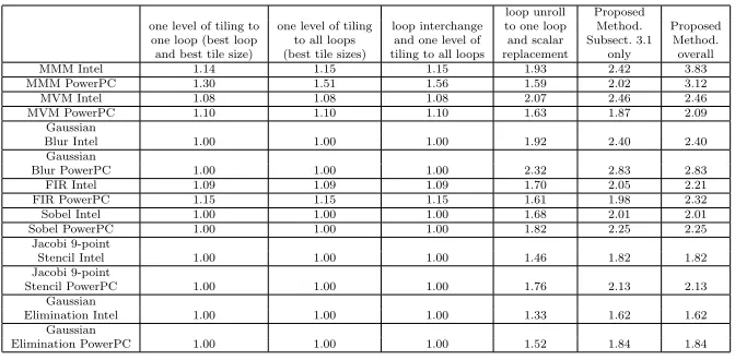
Table 2 Performance evaluation for fixed input sizes (those of Table 1). The speedup values refer to the ratio of the benchmark code execution time to the transformed code execution time (gcc compiler is used).

loop unroll Proposed

one level of tiling to one level of tiling loop interchange to one loop Method. Proposed one loop (best loop to all loops and one level of and scalar Subsect. 3.1 Method. and best tile size) (best tile sizes) tiling to all loops replacement only overall MMM Intel 1.14 1.15 1.15 1.93 2.42 3.83 MMM PowerPC 1.30 1.51 1.56 1.59 2.02 3.12 MVM Intel 1.08 1.08 1.08 2.07 2.46 2.46 MVM PowerPC 1.10 1.10 1.10 1.63 1.87 2.09

Gaussian

Blur Intel 1.00 1.00 1.00 1.92 2.40 2.40 Gaussian

Blur PowerPC 1.00 1.00 1.00 2.32 2.83 2.83 FIR Intel 1.09 1.09 1.09 1.70 2.05 2.21 FIR PowerPC 1.15 1.15 1.15 1.61 1.98 2.32 Sobel Intel 1.00 1.00 1.00 1.68 2.01 2.01 Sobel PowerPC 1.00 1.00 1.00 1.82 2.25 2.25

Jacobi 9-point

Stencil Intel 1.00 1.00 1.00 1.46 1.82 1.82 Jacobi 9-point

Stencil PowerPC 1.00 1.00 1.00 1.76 2.13 2.13 Gaussian

Elimination Intel 1.00 1.00 1.00 1.33 1.62 1.62 Gaussian

Elimination PowerPC 1.00 1.00 1.00 1.52 1.84 1.84

and d) loop unroll to one loop and scalar replacement (best loop and best unroll factor value) (Table 2). Given that even the search space of the (a)-(d) above is huge, only one different set of input sizes is used (the input sizes are those shown in Table 1). Moreover, the number of different tile sizes tested here are limited (from 1 up to 2 orders of magnitude smaller than those used to estimate Table 1). Even for a limited input and tile sizes the number of different binaries is large and thus the experimental results of Table 2 took several days.

(20)

(L/S) and addressing instructions. However, it does not take into account data reuse and the number of registers and this is why the methodology given in Subsect. 3.1 performs about 1.25 times faster. As it was expected, by unrolling the innermost loops, performance is not highly increased since the data reuse being achieved is low.

As it was expected, one level of loop tiling is not performance efficient for Gaussian Blur, Sobel and Jacobi Stencil since the locality advantage is lost by the additional addressing (tiling adds more loops) and load/store instructions (there are overlapping array elements which are loaded twice [55]). Regarding Gaussian Elimination, loop tiling is not performance efficient because the loops allowed to be tiled (data dependencies) a) do not have fixed bound values (data reuse is decreased in each iteration), b) the upper row of the matrix (which is reused many times) always fits in L1. This is why the methodology given in Subsect. 3.1 achieves the best observed speedup for the Gaussian Blur, Sobel, Jacobi Stencil and Gaussian Elimination.

Regarding MMM, MVM and FIR, loop tiling is performance efficient, es-pecially, when it is applied according to Subsect. 3.2; Subsect. 3.2 applies loop tiling in a more efficient way (it takes into account data reuse, memory architecture details and data array layouts) giving higher speedup values. Re-garding MMM, loop tiling is performance efficient for matrix sizes larger than

90×90 for both processors (both processors contain 32kbyte L1 data cache).

At the MVM case, loop tiling is performance efficient for matrix sizes larger than 4096×4096. As far as FIR is concerned, loop tiling is effective for filter sizes larger than 4000.

Loop tiling is more efficient on PowerPC processor because PowerPC con-tains only one level of cache, making the memory management problem more critical. In contrast to MMM, the MVM and the FIR do not increase their performance by applying loop tiling to more than one loop iterator; this is because MMM contains three very large arrays and one extra iterator, making loop tiling transformation more critical. As far as loop interchange transfor-mation is concerned, it does not increase performance except from MMM in PowerPC (I believe that gcc already applies loop interchange, at least on Intel processor).

Moreover, an evaluation over gcc/icc compilers is made. Icc performs better than gcc, for all algorithms. A large number of different input sizes is tested for each algorithm and the average speedup value is computed. As the input size increases, the speedup slightly increases; this is because loop tiling becomes more critical in this case. It is important to say that by slightly changing the input size, the output schedule changes. The input sizes are the following. For

MMM square matrices of sizes (64×64−4000×4000) are used while for MVM

a square matrix of size (256×256−160000×16000) is used. For Gaussian

Blur, Sobel, Jacobi Stencil and Gaussian Elimination square matrices of sizes

(256×256−3000×3000) are used. Regarding FIR, (array size, filter size) =

(21)

[image:21.595.72.415.106.219.2]

Table 3 Performance comparison over gcc 4.8.4, icc 2015 and PowerPC compilers

I ntelX eonE₃−1240v3

Average MMM MVM Gaussian FIR Sobel Jacobi 9-point Gaussian

Speedup Blur Stencil Elimination

gcc 3.₃ ₂.₅ ₂.₃ ₂.₀ ₁.₉ ₁.₈ ₁.₆

icc 2.5 1.9 2.1 1.6 1.5 1.4 1.3

P owerP C₄₄₀

Average MMM MVM Gaussian FIR Sobel Jacobi 9-point Gaussian

Speedup Blur Stencil Elimination

PowerPC 2.₆ ₁.₉ ₂.₇ ₂.₀ ₂.₂ ₁.₉ ₁.₈

compiler

The proposed methodology achieves significant speedup values on both processors (Table 3), as the number of load/store instructions and cache ac-cesses is highly decreased. icc applies more efficient transformations than gcc to the benchmark codes, resulting in faster binary code. It is important to say that although icc generates much faster binaries than gcc regarding the benchmark codes, both compilers give close execution time binaries regarding the proposed methodology output codes; this is because both compilers are not able to apply high level transformations at the latter case.

Regarding Intel processor, gcc and icc compilers generate binary code con-taining SSE/AVX instructions (auto-vectorization) and thus they use 256-bit / 128-bit YMM / XMM registers. However, the proposed methodology does not support auto-vectorization (it is out of the scope of this paper); thus, all the benchmark C-codes that used on Intel, use SSE instrinsics. In this way, both input and output codes contain the SSE instrinsics. As far as the PowerPC processor is concerned, benchmark C-codes do not contain vector instructions. The best observed speedup for Intel processor is achieved for MMM while the best speedup for PowerPC is achieved for Gaussian Blur and MMM (Ta-ble 3). MMM achieves the largest speedup values because it contains three very large 2-d arrays providing data reuse (loop tiling has a larger effect in such cases). The MMM schedules that achieve best performance on Intel include loop tiling for L1 and L3 and tile-wise data array layouts for A and B, when

C =C+A×B (when the input size is large enough). The MMM schedules

that achieve best performance on PowerPC include tiling for L1 data cache and tile-wise layouts for the arrays A and B. Moreover, the methodology given in Subsect. 3.1, has a very large effect on performance for both processors (Table 1).

Regarding MVM (Table 3), speedup of 2.5 and 1.9 is achieved for Intel

and PowerPC, respectively. Loop tiling for cache is not performance efficient for Intel processor (speedup lower than 1%) since the total size of the arrays

that achieve data reuse is small (Y and X arrays, when Y = Y +A×X)

and they fit in fast L2 cache in most cases. However, PowerPC has one level of data cache only and thus loop tiling is performance efficient for large array

(22)

not performance efficient to be changed for two reasons (at both processors). First, array A size is very large compared to the X and Y ones and second, A

is not reused (each element ofAis accessed only once).

Regarding Gaussian Blur, a large speedup value is achieved in both cases.

Gaussian Blur contains two 2-d arrays (images) and a 5×5 mask array which is

always shifted by one position to the right to the input image. The input image and the mask array achieve data reuse and thus both array elements are as-signed into registers. Regarding Intel processor, the speedup values are 2.3 and 2.1 for gcc and icc, respectively, while for PowerPC the highest speedup value is achieved, i.e., 2.7. Loop tiling is performance efficient only for very large input sizes. As far as PowerPC is concerned, it achieves a larger speedup value than Intel because by creating a large loop body, compilers apply scalar replacement to the Gaussian mask elements, decreasing the number of load/store and arith-metical instructions; the decreased number of instructions has a larger effect on the smaller PowerPC processor which contains only one ALU unit.

FIR achieves a significant but not large performance gain (Table 3) because FIR arrays are of small size. In the case that L1 data cache size is smaller than twice the size of the filter array, loop tiling is necessary. This is because the filter array and a part of the input array (they are of the same size) are loaded in each iteration; if L1 is smaller than this value, the filter array cannot remain in L1 and thus it is fetched many times from the upper memory. In this case loop tiling for L1 is performance efficient; loop tiling is not applied for Intel L2/L3 cache memories since the total size of the arrays is smaller here.

In Sobel Operator two 3×3 mask arrays are applied to the input

im-age, shifted by one position to the right. I use the Manhattan instead of Eu-clidean distance because in the latter case performance highly depends on the Euclidean distance computation (especially on PowerPC); I use if-condition

statements instead ofatan() functions for the same reason. PowerPC achieves

a larger speedup value than Intel because by increasing the loop body size, compiler apply scalar replacement to the Sobel mask elements (Sobel mask el-ements contain only ones and zeros), decreasing the number of load/store and arithmetical instructions; the decreased number of instructions has a larger effect on the smaller PowerPC processor which contains only one ALU unit.

Regarding Jacobi 9-point Stencil, speedup values are 1.7 and 1.4 over gcc and icc, respectively (Intel processor). As far as PowerPC is concerned, a larger

speedup value is achieved (1.9). Data reuse is achieved in each iteration for

the six of the nine array elements which are assigned into registers. Three loads occur in each iteration and not nine, since six registers interchange their values as in (Fig. 3-(d)). Regarding Intel processor, data reuse is achieved by computing more than one result (from vertical dimension) in each iteration.

(23)

5 Conclusions

In this paper, six compiler optimizations are addressed together as one problem and not separately, for a wide range of algorithms and computer architectures. New methods for loop unroll and loop tiling are given which take into account the custom SW characteristics and the HW architecture details. In this way, the search space is decreased by many orders of magnitude and thus it is capable to be searched.

References

1. S. Triantafyllis, M. Vachharajani, N. Vachharajani, D. I. August, Compiler optimization-space exploration, in: Proceedings of the international symposium on Code generation and optimization: feedback-directed and runtime optimization, CGO ’03, IEEE Com-puter Society, Washington, DC, USA, 2003, pp. 204–215.

URLhttp://dl.acm.org/citation.cfm?id=776261.776284

2. K. D. Cooper, D. Subramanian, L. Torczon, Adaptive Optimizing Compilers for the 21st Century, Journal of Supercomputing 23 (2001) 2002.

3. T. Kisuki, P. M. W. Knijnenburg, M. F. P. O’Boyle, F. Bodin, H. A. G. Wijshoff, A Feasibility Study in Iterative Compilation, in: Proceedings of the Second International Symposium on High Performance Computing, ISHPC ’99, Springer-Verlag, London, UK, UK, 1999, pp. 121–132.

4. P. A. Kulkarni, D. B. Whalley, G. S. Tyson, J. W. Davidson, Practical Exhaustive Op-timization Phase Order Exploration and Evaluation, ACM Trans. Archit. Code Optim. 6 (1) (2009) 1:1–1:36. doi:10.1145/1509864.1509865.

URLhttp://doi.acm.org/10.1145/1509864.1509865

5. P. Kulkarni, S. Hines, J. Hiser, D. Whalley, J. Davidson, D. Jones, Fast searches for effective optimization phase sequences, SIGPLAN Not. 39 (6) (2004) 171–182. doi:10.1145/996893.996863.

URLhttp://dl.acm.org/citation.cfm?doid=996893.996863

6. E. Park, S. Kulkarni, J. Cavazos, An evaluation of different modeling techniques for iterative compilation, in: Proceedings of the 14th international conference on Compilers, architectures and synthesis for embedded systems, CASES ’11, ACM, New York, NY, USA, 2011, pp. 65–74. doi:10.1145/2038698.2038711.

7. A. Monsifrot, F. Bodin, R. Quiniou, A Machine Learning Approach to Automatic Pro-duction of Compiler Heuristics, in: Proceedings of the 10th International Conference on Artificial Intelligence: Methodology, Systems, and Applications, AIMSA ’02, Springer-Verlag, London, UK, UK, 2002, pp. 41–50.

8. M. Stephenson, S. Amarasinghe, M. Martin, U.-M. O’Reilly, Meta optimization: im-proving compiler heuristics with machine learning, SIGPLAN Not. 38 (5) (2003) 77–90. doi:10.1145/780822.781141.

9. M. Tartara, S. Crespi Reghizzi, Continuous learning of compiler heuristics, ACM Trans. Archit. Code Optim. 9 (4) (2013) 46:1–46:25. doi:10.1145/2400682.2400705.

10. F. Agakov, E. Bonilla, J. Cavazos, B. Franke, G. Fursin, M. F. P. O’Boyle, J. Thomson, M. Toussaint, C. K. I. Williams, Using Machine Learning to Focus Iterative Optimiza-tion, in: Proceedings of the International Symposium on Code Generation and Opti-mization, CGO ’06, IEEE Computer Society, Washington, DC, USA, 2006, pp. 295–305. doi:10.1109/CGO.2006.37.

(24)

11. L. Almagor, K. D. Cooper, A. Grosul, T. J. Harvey, S. W. Reeves, D. Subramanian, L. Torczon, T. Waterman, Finding Effective Compilation Sequences, SIGPLAN Not. 39 (7) (2004) 231–239. doi:10.1145/998300.997196.

12. K. D. Cooper, P. J. Schielke, D. Subramanian, Optimizing for Reduced Code Space Us-ing Genetic Algorithms, SIGPLAN Not. 34 (7) (1999) 1–9. doi:10.1145/315253.314414. URLhttp://doi.acm.org/10.1145/315253.314414

13. K. D. Cooper, A. Grosul, T. J. Harvey, S. Reeves, D. Subramanian, L. Torczon, T. Wa-terman, ACME: Adaptive Compilation Made Efficient, SIGPLAN Not. 40 (7) (2005) 69–77. doi:10.1145/1070891.1065921.

14. K. D. Cooper, A. Grosul, T. J. Harvey, S. Reeves, D. Subramanian, L. Torczon, T. Wa-terman, Exploring the Structure of the Space of Compilation Sequences Using Random-ized Search Algorithms, J. Supercomput. 36 (2) (2006) 135–151. doi:10.1007/s11227-006-7954-5.

URLhttp://dx.doi.org/10.1007/s11227-006-7954-5

15. P. Kulkarni, S. Hines, J. Hiser, D. Whalley, J. Davidson, D. Jones, Fast Searches for Effective Optimization Phase Sequences, SIGPLAN Not. 39 (6) (2004) 171–182. doi:10.1145/996893.996863.

16. P. A. Kulkarni, D. B. Whalley, G. S. Tyson, Evaluating Heuristic Optimization Phase Order Search Algorithms, in: Proceedings of the International Symposium on Code Generation and Optimization, CGO ’07, IEEE Computer Society, Washington, DC, USA, 2007, pp. 157–169. doi:10.1109/CGO.2007.9.

URLhttp://dx.doi.org/10.1109/CGO.2007.9

17. C. Chen, J. Chame, M. Hall, Combining Models and Guided Empirical Search to Opti-mize for Multiple Levels of the Memory Hierarchy, Proceedings of the 2013 IEEE/ACM International Symposium on Code Generation and Optimization (CGO) 0 (2005) 111– 122. doi:10.1109/CGO.2005.10.

18. M. Haneda, P. M. W. Khnijnenburg, H. A. G. Wijshoff, Automatic Selection of Compiler Options Using Non-parametric Inferential Statistics, in: Proceedings of the 14th International Conference on Parallel Architectures and Compilation Techniques, PACT ’05, IEEE Computer Society, Washington, DC, USA, 2005, pp. 123–132. doi:10.1109/PACT.2005.9.

URLhttp://dx.doi.org/10.1109/PACT.2005.9

19. F. Agakov, E. Bonilla, J. Cavazos, B. Franke, G. Fursin, M. F. P. O’Boyle, J. Thomson, M. Toussaint, C. K. I. Williams, Using Machine Learning to Focus Iterative Optimiza-tion, in: Proceedings of the International Symposium on Code Generation and Opti-mization, CGO ’06, IEEE Computer Society, Washington, DC, USA, 2006, pp. 295–305. doi:10.1109/CGO.2006.37.

20. J. Cavazos, G. Fursin, F. Agakov, E. Bonilla, M. F. P. O’Boyle, O. Temam, Rapidly Selecting Good Compiler Optimizations Using Performance Counters, in: Proceedings of the International Symposium on Code Generation and Optimiza-tion, CGO ’07, IEEE Computer Society, Washington, DC, USA, 2007, pp. 185–197. doi:10.1109/CGO.2007.32.

21. F. de Mesmay, Y. Voronenko, M. P¨uschel, Offline Library Adaptation Using Auto-matically Generated Heuristics, in: International Parallel and Distributed Processing Symposium (IPDPS), 2010, pp. 1–10.

22. C. Dubach, T. M. Jones, E. V. Bonilla, G. Fursin, M. F. P. O’Boyle, Portable Com-piler Optimisation Across Embedded Programs and Microarchitectures Using Ma-chine Learning, in: Proceedings of the 42Nd Annual IEEE/ACM International Sym-posium on Microarchitecture, MICRO 42, ACM, New York, NY, USA, 2009, pp. 78–88. doi:10.1145/1669112.1669124.

(25)

24. D. Kim, L. Renganarayanan, D. Rostron, S. Rajopadhye, M. M. Strout, Multi-level Tiling: M for the Price of One, in: Proceedings of the 2007 ACM/IEEE Confer-ence on Supercomputing, SC ’07, ACM, New York, NY, USA, 2007, pp. 51:1–51:12. doi:10.1145/1362622.1362691.

25. L. Renganarayanan, D. Kim, S. Rajopadhye, M. M. Strout, Parameterized Tiled Loops for Free, SIGPLAN Not. 42 (6) (2007) 405–414. doi:10.1145/1273442.1250780. URLhttp://doi.acm.org/10.1145/1273442.1250780

26. G. Fursin, M. F. P. O’Boyle, P. M. W. Knijnenburg, Evaluating iterative compilation, in: Languages and Compilers for Parallel Computing, 15th Workshop, (LCPC) 2002, College Park, MD, USA, July 25-27, 2002, Revised Papers, 2002, pp. 362–376. 27. H. Leather, E. Bonilla, M. O’Boyle, Automatic Feature Generation for Machine Learning

Based Optimizing Compilation, in: Proceedings of the 7th Annual IEEE/ACM Interna-tional Symposium on Code Generation and Optimization, CGO ’09, IEEE Computer Society, Washington, DC, USA, 2009, pp. 81–91. doi:10.1109/CGO.2009.21.

28. M. Stephenson, S. Amarasinghe, Predicting Unroll Factors Using Supervised Classifi-cation, in: Proceedings of the International Symposium on Code Generation and Opti-mization, CGO ’05, IEEE Computer Society, Washington, DC, USA, 2005, pp. 123–134. doi:10.1109/CGO.2005.29.

29. E. Park, L.-N. Pouche, J. Cavazos, A. Cohen, P. Sadayappan, Predictive Modeling in a Polyhedral Optimization Space, in: Proceedings of the 9th Annual IEEE/ACM Inter-national Symposium on Code Generation and Optimization, CGO ’11, IEEE Computer Society, Washington, DC, USA, 2011, pp. 119–129.

30. M. R. Jantz, P. A. Kulkarni, Exploiting Phase Inter-dependencies for Faster Iterative Compiler Optimization Phase Order Searches, in: Proceedings of the 2013 International Conference on Compilers, Architectures and Synthesis for Embedded Systems, CASES ’13, IEEE Press, Piscataway, NJ, USA, 2013, pp. 7:1–7:10.

31. S. Kulkarni, J. Cavazos, Mitigating the Compiler Optimization Phase-ordering Problem Using Machine Learning, SIGPLAN Not. 47 (10) (2012) 147–162. doi:10.1145/2398857.2384628.

32. E. Park, S. Kulkarni, J. Cavazos, An Evaluation of Different Modeling Techniques for Iterative Compilation, in: Proceedings of the 14th International Conference on Compil-ers, Architectures and Synthesis for Embedded Systems, CASES ’11, ACM, New York, NY, USA, 2011, pp. 65–74. doi:10.1145/2038698.2038711.

33. D. Parello, O. Temam, A. Cohen, J.-M. Verdun, Towards a Systematic, Pragmatic and Architecture-Aware Program Optimization Process for Complex Processors, in: Proceedings of the 2004 ACM/IEEE Conference on Supercomputing, SC ’04, IEEE Computer Society, Washington, DC, USA, 2004, pp. 15–. doi:10.1109/SC.2004.61. URLhttp://dx.doi.org/10.1109/SC.2004.61

34. H. Rong, A. Douillet, G. R. Gao, Register Allocation for Software Pipelined Multi-dimensional Loops, SIGPLAN Not. 40 (6) (2005) 154–167. doi:10.1145/1064978.1065030.

35. S. Hack, G. Goos, Optimal Register Allocation for SSA-form Programs in Polynomial Time, Inf. Process. Lett. 98 (4) (2006) 150–155. doi:10.1016/j.ipl.2006.01.008. URLhttp://dx.doi.org/10.1016/j.ipl.2006.01.008

36. S. G. Nagarakatte, R. Govindarajan, Register Allocation and Optimal Spill Code Scheduling in Software Pipelined Loops Using 0-1 Integer Linear Programming Formu-lation, in: Proceedings of the 16th International Conference on Compiler Construction, CC’07, Springer-Verlag, Berlin, Heidelberg, 2007, pp. 126–140.