Shape descriptors and mapping methods for full field comparison of experimental to simulation data

Shape descriptors and mapping methods for full-field

comparison of experimental to simulation data

PASIALIS, Vasileios <http://orcid.org/0000-0002-2346-3505> and LAMPEAS,

George

Available from Sheffield Hallam University Research Archive (SHURA) at:

http://shura.shu.ac.uk/11877/

This document is the author deposited version. You are advised to consult the

publisher's version if you wish to cite from it.

Published version

PASIALIS, Vasileios and LAMPEAS, George (2015). Shape descriptors and mapping

methods for full-field comparison of experimental to simulation data. Applied

Mathematics and Computation, 256, 203-221.

Copyright and re-use policy

See

http://shura.shu.ac.uk/information.html

Sheffield Hallam University Research Archive

1.

Introduction

The optimization of modern engineering structures takes advantage of structural simulation and material developments, which however cannot be fully exploited without a rigorous validation of simulations with respect to experimental results.

Current practice to demonstrate structural reliability and provide confidence in the design and simulation processes tends to focus on identifying hot-spots in the data and check that the experimental and modeling results have a satisfactory agreement in these critical zones. Often the comparison is even restricted to a single point where the maximum stress occurs. This highly localized approach is the result of the traditional strain measurement approaches performed by strain gauges, but neglects the majority of data generated by numerical analysis and full-field measurement techniques, carrying with it the risk that critical regions may be missed all together [1].

Recently, full-field optical displacement / strain measurement techniques have been developed up to a technology readiness level, such that they can reliably capture the higher part or even the entire structural field during an experimental test. Full-field optical techniques provide a useful tool for the deeper understanding of deformation and failure process of structural elements, as well as it can be used in the assessment of the

accuracy of numerical simulation results by comparing predicted values to corresponding experimental data [2]. The strength of full-field optical methodologies is that the entire displacement field can be visualized and analyzed. As a result, Digital Image Correlation (DIC), Moiré, holographic and Digital Speckle Pattern Interferometry (DSPI) or shearography, steadily replace conventional measurement techniques such as strain gauges, extensometers, etc.

Full-field comparison between simulation and experimental results often requires transform techniques to reduce the high amount of ‘raw’ data to a fairly modest number of features. These descriptors retain most of the useful information and facilitate the comparison of experimental deformation captured by full-field optical measurement systems to the respective simulation results, e.g. [3] and [4].

Various polynomials exist in the literature, which can be used to decompose images [5, 6]; some of them can be applied to transform displacement and strain plots obtained by optical measurement systems or

calculated by simulation, in order to enable a comparison between them. The continuous Zernike and

Chebyshev polynomials are particularly suitable for the transform process, because of their unique properties, such as orthogonality and accurate reconstruction of the digital image. Other important properties include invariance to transformations (rotation, translation, scale), good rate of convergence, noise reduction, easiness of programming and applicability for comparison purposes (i.e. good compaction using few moment terms). Moreover, the reconstruction accuracy can further be improved as shown in ref. [7] by using some well-known numerical integration techniques. Taking into account that Zernike polynomials are defined in the unit disc space, they are ideally suited to circular shaped structures [8], while Chebyshev polynomials [9] are better suited to rectangular domains. In order to apply Zernike polynomials to other geometries, the non-circular shape should initially be mapped onto a unit disc space. Various mapping techniques have been applied in the literature e.g. [10, 11, 12]. In any case, the magnitudes and number of Zernike moment terms required to describe the circular image depend on the applied mapping technique.

The efficiency of each approach in data compaction and data pre-processing for comparison purposes is assessed. For this scope, four different mappings of a rectangular surface to a unit disc are applied, followed by Zernike transform, and their results are compared against a continuous Chebyshev transform. A deep

mathematical investigation to the reasons of the different performance of the four mapping methods has been performed, comprising the effects of image mapping distortion and the numerical integration accuracy.

the present investigation that compared to Chebyshev polynomials, Zernike shape descriptors can be more efficient even in cases of non-circular shapes and patterns, as long as the appropriate mapping is selected.

2.

Orthogonal transform polynomials and mapping methods

transform

In the present paper, transform of non-circular data fields is performed by applying Zernike polynomials combined to appropriate mappings, as well as Chebyshev polynomials of the second kind. Despite the fact that the Chebyshev polynomials of the first kind are generally used, Chebyshev polynomials of the second kind have been applied here, as they have been proven appropriate for the image decomposition / reconstruction process and satisfy some exciting identities as mentioned in [13]. The monomial basis is employed in Chebyshev computation, in order to have the same analytic expression of orthogonal moments for both Zernike and Chebyshev polynomials (eq. 1, 2) and to use the same programming procedures.

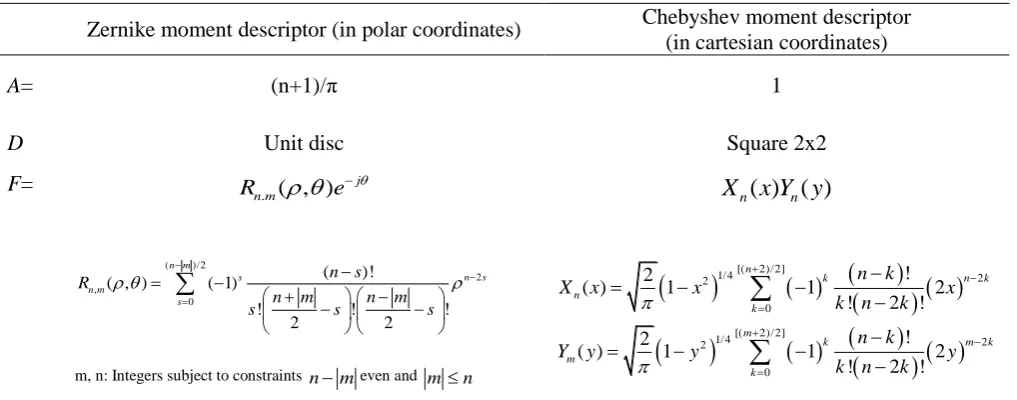
The general form of Zernike and Chebyshev moment descriptors in continuous orthogonal basis are described by Eqs. 1, 2:

, ( , ) , ( , )

n m _D n m

M  A



, ( , ) , ( , )

n m _D n m

M A



 

    

In eq. (1) and (2), D is the spatial domain of (x, y) variables, A is a constant depending on the shape descriptor, I denotes the continuous shape pattern (in the present case displacement or strain) and F is the shape polynomial, often described as transformation kernel. In the following Table 1, the above parameters are provided, for the cases ofZernike and Chebyshev moment descriptors.

Zernike moment descriptor (in polar coordinates) Chebyshev moment descriptor (in cartesian coordinates)

A= (n+1)/π 1

D Unit disc Square 2x2

F=

. ( , ) j n m

R   e

( )/ 2

2 ,

0

( )!

( , ) ( 1)

! ! !

2 2

n m

s n s

n m

s

n s R

n m n m

s s s

                        



m, n: Integers subject to constraints _n_meven and _m_n

( ) ( )

n n

X x Y y





  





  





  





  

[( 2)/ 2]

1/ 4 2

2 0 [( 2)/ 2]

1/ 4 2

2 0

! 2

( ) 1 1 2

! 2 !

! 2

( ) 1 1 2

! 2 !

n

k n k

n

k m

k m k

m

k

n k

X x x x

k n k n k

Y y y y

k n k

                 





Table 1: Zernike and Chebyshev moment descriptor variables

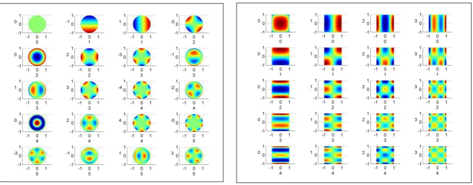
Figure 1: Zernike polynomials (left) and second kind Chebyshev polynomials (right).

The full field data I may be expressed as a linear combination of orthonormal kernel functions as:

, , n m n m n m

I

M

F

 





(Eq.3)

However, as the reconstruction of an image using infinite number of shape descriptors is not practically possible, an efficient approximate reconstruction may be achieved by keeping in the equation only the moments and their relative shape polynomials of the higher value, while the remaining terms are discarded. In Eq. (4) I is the approximated reconstructed image.

, , N M

n m n m n m

I





M

F

In case of Zernike moments, rotation invariance may be exploited by calculating only the positive terms (m≥0) resulting in the following equation:



 



, 0

0

2

( ) Re

cos(

) Im

sin(

)

Re

Im

( )

N M

n m n m n n

n m n

n m

I

R



M

m



M

m



M

j

M

R















































In order to minimize numerical integration errors, a convergence analysis was carried out, which resulted in a quite high number of interpolation points, i.e. 501 points per dimension and 251001 points in total. Using the moment transform approach, a map / image containing thousands or millions of nodes / pixels may be described by few moment descriptor terms.The quality of the reconstruction depends on the number of shape moments retained in the image reconstruction, the selection of which can be determined by using a predefined threshold when comparing the similarity between the original image / map and its numerically reconstructed counterpart. Further condensation is performed by retaining only the most important moments among those initially computed. The measure of a moment’s contribution to the image description is its magnitude, therefore only the greatest moment magnitudes are retained. It should be noted here that the input to the analysis is raw data in vector form, as extracted from the FE simulations and the DIC measurement system; images are created afterwards from these data using a Matlab code. In case that images are preferable instead of raw data,

The accuracy of the shape moment approximation can be evaluated using different expressions. The most common equations are the Normalized Root Mean Square error (NRMS) [8] in the form of Eq.6 and the

Correlation Coefficient in the form of Eq.7, [11].

[

]

I x y I x y dxdy e

I x y dxdy

∬

∬

where,

I x y

( , )

 

 

 





ˆ ˆ ˆ

ˆ ˆ ( , )

I I I I dA corr I I

I I dA I I dA

       _{    }  _{  }  

∬

∬

∬

In eq. (6) and (7),

ˆ

ˆ

IdA

I

dA



∬

∬

IdA

I

dA



∬

∬

2.2 Unit disc mapping techniques

The Zernike moments are defined in a unit disc. Therefore, any image data must be mapped onto a unit disc before executing the data condensation process. Four different mapping techniques (referred to as mapping A, B, C and D) of a flat rectangular to a flat unit disc are investigated and their results are compared against each other.

A displacement / strain map usually is not a random pattern. For instance, impact loadings create circular or oval patterns around the impact event, tensile tests create locally uniform displacement, metal forming processes often create oval shapes, etc. Any map / image will be described with a relatively small number of moments, if it resembles enough some of the transformation kernels depicted in Figure 1.

By observing the images of Figure 1, it is evident that Zernike moment descriptor describes efficiently circular patterns, whereas Chebyshev moment descriptor better suits to rectangular patterns. However, in the case of Zernike moments, the way information is mapped to the unit disc seriously affects the performance of the subsequent data transform process. Therefore, any mapping which creates discontinuities or alters the original shape into a pattern non-resembling the Zernike shape polynomials is expected to lead to an increase in the number of moments used for efficient data condensation.

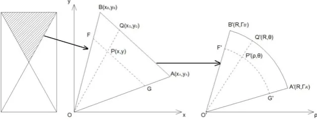
Figure 2: Schematical representation of Mapping A.

The mapping of the rectangle to the circular sector is performed by using eqs. (8, 9)

2 2 2 2

/ 2

(Eq.8)

θ=arctan (Eq.9)

a a

b b

a

a

x y a

r

x y

y x

  



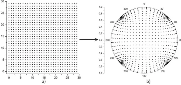
Another known way to map a rectangle to a unit disk, referred hereafter as Mapping B, is presented in Figure 3, in which the points of square perimeters are uniformly distributed along circular perimeters [12]. The previous steps include the normalization of the rectangular image to the square image and the acquirement of a new dataset of uniformly distributed interpolated points.

Figure 3: Schematical representation of Mapping B.

Figure 4: Schematical representation of Mapping C.

The following equations express the new coordinates of the points mapped inside the unit disc in polar coordinates (eq, 9,10):



 



A B B A

y y x x x y

R x y x y





(Eq.9)



 

 



A A

B A B A

xy

x y

y

y

x

x

x

y







  

 







(Eq.10)

A fourth mapping approach, investigated presently, is the conformal mapping taken from ref [17]. Such a mapping technique preserves angles between arcs in the domain and image (hence the name conformal). This conformal mapping method represents the original shape features more efficiently without creating

discontinuities in the final map. The roots of conformal mapping lie early in the nineteenth century. The

Schwarz-Christoffel (SC) conformal formula was discovered independently by Christoffel in 1867 and Schwarz in 1869 [16] and was still under investigation until the end of the twentieth century, when numerical

computation of varied SC transformations was feasible with the use of computers. The square to unit disc mapping, however, is rather an easy case.

A typical SC mapping is depicted in Figure 5, from which four very dense clusters of points may be observed, making SC mapping ideal in quarter-symmetry models when there is a lot of fine information in one corner of the map. Nevertheless, it worth to be noted that these four cluster points did not create any problems with respect to smoothness or reconstruction error, as it may be observed in the demonstration examples of section 3. The interpolation points on the square are given by eqs. 12 and 13, while eqs. 14 and 15 calculate the polar coordinates of the corresponding points on the unit disc.

Figure 5: Schematical representation of Mapping D; Schwarz-Christoffel (SC) conformal transformation of a square to the unit disc.

2 1

cos , 0,1, 2,..., (Εq.12)

2 2

2 1

cos , k=0,1,2,...,N

2 2

j

k

j

x j M

M k y N





  (Eq.13)

coslem exp(

/ 4)

(

1

) (Εq.14)

2

angle coslem exp(

/ 4)

(

1

(Eq.15)

2

jk j k

jk j k

K

r

x

iy

i

K

x

iy

i



















 

























 













where coslem is the cosine-lemniscate function, given by Eq.16

 









coslem( ) 1.1981402

1 sech 1.1981402

2.6220576

(Eq.16)

m

m













3.

Transform of numerically calculated displacement and strain images

Four properly selected demonstration cases, comprising a monolithic flat plate subjected to low-velocity impact, a simple tensile specimen under static loading, an impacted honeycomb sandwich panel and a sheet metal forming problem are selected for the investigation on the different mapping / transform techniques. Transform techniques are applied in order to reduce the high amount of ‘raw’ data to a fairly modest number of features, while retaining all essential information of the image. Comparison with the respective experimental features, or other procedures may be performed subsequently.

3.1 Monolithic flat panel under low-velocity impact

Figure 6: Numerical model of a monolithic plate under low-velocity central impact; upper side and impactor (left) and lower sideand spherical supports (right).

The spherical supports are modeled as infinite mass rigid walls, while the impactor is modeled as a rigid body with one degree of freedom in the direction of impact. The plate comprises 5220 quad-shell elements. Node-to-surface contact type is used to model the contact of the rigid parts to the deformable plate. The

behaviour of the plate is described by a bilinear elastoplastic material model with failure. Displayed in Figure 7 is the out-of-plane displacement map after 2ms of impact. In Figure 8, mapping results calculated by the four different mappings A to D are presented. It may be observed from Figure 8, that the results obtained by mapping techniques A, B and C generate discontinuities, which may hinder the image further transform by continuous functions, in contrast to the Schwarz-Christoffel mapping D (Figure 8d).

Figure 7: Out-of-plane displacement map of impacted monolithic plate, 2ms after impact.

Figure 8: Monolithic flat plate mapping results by a) Mapping A b) Mapping B c) Mapping C d) Mapping D (SC).

The square plot of Figure 7, as well as the four circular plots obtained by the four mapping methods, (Figure 8) are decomposed by Chebyshev and Zernike moment descriptors, respectively. Consequently, the original images are reconstructed by eq. (6), using a number of finite terms. As mentioned above, the retained number of terms may be selected by comparing the original and the reconstructed image by means of the NRMS error (eq. 6) or Correlation Coefficient (eq 7).

This case is also appropriate to demonstrate the differences of the two aforementioned expressions (Eqs. 6-7) in assessing the reconstruction error. Displayed in Figure 9 is image description with Zernike moments and SC mapping. In Figure 9(left) and (right) the reconstruction error (1%) is evaluated with the NRMS error and the Correlation Coefficient, respectively. From Figure 9 it is obvious that the Correlation Coefficient (Eq.7) evaluates the image approximation in a less rigorous manner than the other equation (Eq.6). In this case, 15% in Normalized Root Mean Square error corresponds to 1% in Correlation Coefficient (Figure 9) ; the same

observation is also illustrated in Figure 10, in which the NRMS and corelation errors are plotted against the number of retained transform terms.

Figure 10: Comparison between the two basic expressions used for the assessment of image reconstruction error. The Correlation Coefficient (corr) goes to steady-state condition must faster than the Nomalized Root Mean Square error (e).

For this reason, and although the Correlation Coefficient (eq. 7), is commonly used in optical character and fingerprint recognition, the NRMS error indicator is selected as the more appropriate norm in all cases studied hereafter to help in the selection of image transform retained terms.

3.2 Tensile specimen under static loading

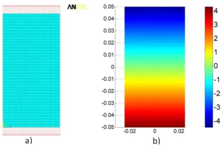
Tensile tests of simple flat specimens are commonly used to access the mechanical properties of materials. A simple Finite Element model of the central section of a tensile specimen, consisting of shell elements is created in order to calculate the displacement field, as presented in Figure 11.

In Figure 12, mapping results calculated by the four investigated mapping techniques are presented. Mappings using techniques A, B and C as presented in Figure 12a-c reveal that the initial shape pattern has been split to four distinguishable parts, therefore, creating discontinuities at their mutual borders. In contrast,

mapping D (SC mapping) presented in Figure 12d retains the shape pattern of the original image and does not generate any discontinuity.

Figure 12: Tensile specimen displacement mapping results by a) Mapping A b) Mapping B c) Mapping C d) Mapping D (SC).

3.3 Honeycomb sandwich impacted panel

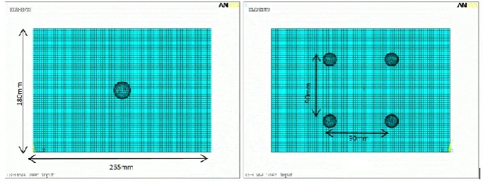
Honeycomb sandwich panels are commonly used in aerospace structures. Typical loading conditions include low and high velocity impact events on the panel surface (skin) by space debris. Finite Element simulation of a low-velocity impact event on a honeycomb type sandwich panel has been performed using the explicit dynamic FE code ANSYS-LS DYNA. The model is simply supported by four spheres positioned centrically on the four corners. The spherical supports are modeled as infinite mass rigid walls, while the impactor is modeled as a rigid body with one degree of freedom in the direction of impact. The skin and honeycomb core are modeled using 14600 and 58944 quad-shell elements, respectively.

The quarter-symmetry model is presented in Figure 13. Self-impacting type of contact for core and skins and node-to-surface type for contact of the rigid parts to the skin-core system are used. The failure behavior of the carbon-fiber reinforced epoxy skin is described by the Chang and Chang material model, while the core material is aluminum described by a bilinear elastoplastic material model.

Under investigation is the out-of-plane displacement field of the upper skin. Other parts of the model, especially the internal parts, cannot easily be used for comparison purposes with the respective experimental results, due to the obvious incapacity of optical instruments to acquire measurements.

Figure 13: a) Quarter-symmetry simulation model (small picture) and mesh detail b) Calculated out-of plane displacement 5msafter impact c) Calculated out-of-plane displacement of the upper skin 5ms after impact.

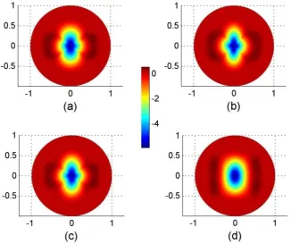
Displayed in Figure 14 are mapping results calculated by the four investigated mappings techniques. As in the previous case, all Zernike mappings, with the exception of SC mapping D, generate discontinuities which may lead to an increase in the number of Zernike moments needed for efficient map description.

Figure 14: a) Sandwich panel mapping results by a) Mapping A b) Mapping B c) Mapping C d) Mapping D (SC).

3.4 Sheet metal forming problem

Innovative manufacturing processes include the sheet metal forming processes to create complex structural parts. The Asymmetrical Incremental Sheet Forming (AISF) method, in which a rigid spherical tool introduces a downward pressure during its movement along a pre-defined path, results to the typical out-of-plane displacement field, such as the one shown in Figure 15. In this case, rectangular shaped patterns are created. Mapping results calculated by the four investigated mapping techniques are depicted in Figure 16. It is observed that mapping techniques A, B and C alter the rectangular patterns to circular, while the SC

Figure 15: Out-of plane displacement field of a sheet formed by the AISF process.

Figure 16: AISF formed panel mapping results obtained by a) Mapping A b) Mapping B c) Mapping C d) Mapping D (SC).

4. Influence of mapping distortion and numerical integration accuracy on reconstruction

efficiency

4.1 Mapping Distortion investigation

A standard methodology to calculate the distortion arising from the transform process of a flat rectangular geometry to a flat disc is not available in the literature. For this purpose an innovative approach is proposed hereafter, which may also be used for the distortion assessment of any mapping procedure. The approach considers the difference of the discrete data points coordinate values, between their initial position on the rectangular shape and their final position on the circular disc. Consider as an example the Mapping method A, as illustrated in Figure 2 of Section 2.2. According to the mapping, the points A and B are displaced to points A' and B', respectively. Using the Cartesian coordinate system xy of Figure 2, the coordinates of any point before the mapping transform are (x, y), while after the mapping the coordinates of the same point become (x+u, y), (x, y+v), where u and v are the point displacements in x- and y -axis, respectively, due to the transform. By employing the first two terms of a Taylor’s series expansion, the components of the displacements of a point can

be determined; thus, the displacement of point A in a direction parallel to the x-axis isu udx x

 

 , while the remaining components are found in an identical manner and are shown in Figure 17.

Figure 17: Differential changes in x-axis and y-axis Cartesian components of the total displacement vector of point A. The change in length of the element AB is defined according to the principles of Elasticity theory as the normal strain εx. Similarly, the change in the angle between two mutually perpendicular lines at any point is

defined as the shear strain. It can be proven by simple geometrical manipulations that the strains relate to displacements according to equations 17-19.

2 2 1 2 x u u

x x x





1

2

u

y

y

y

































































2

u

u u

y

x

x y

x

y



 

















 



 





 

 

where u, υ stand for the displacements along the x-, y-axis, respectively.

It can be proven that as normal strains are associated with changes in length, they result to area (or volumetric in the 3-dimensional space) changes, but they do not distort the initial shape; while shear strains result to shape distortions, as they are associated with changes in angle. Taking these observations into account, the most suitable magnitude to assess the mapping distortion of the original rectangular shape is the shear strain

γxy. In addition to the shear strain γxy, an expression depending on all three components of the displacement

vector can be defined as:

2 2 2

x y xy

U 







(Eq. 17)

(Eq. 18)

It should be noted here, that as the magnitude U is a function of the terms εx, εy and γxy, it expresses the

combined effect of area change plus distortion of the initial shape after the mapping transform and is analogous to the definition of the specific strain energy U in the Elasticity theory. Results from the mapping distortion analysis for the four investigated mapping methods (MapA to MapD) as assessed by Equations (19) and (20), are displayed in Figure 18 and Figure 19.

Figure 19:Mapping distortion assessed by magnitude U for mapping types A, B C and D.

It can be observed from Figure 18 that the distortion of mapD, as expressed by the shear deformation magnitude γxy, is very low compared to the respective distortions of maps A, B, and C and appears only

localised in areas close to the disc perimeter. The distortion of maps B and C are similar to each other and have relatively larger maximum γxy values compared to the other mappings. Comparing MapA to Maps B and C, it

may be observed that in the former case the distortion plot descritizes the unit disc in eight distinguished areas, while in the latter case in four areas, which implies that potentially image decomposition with fewer moment terms can be achieved using MapB and Map C.

Similarly, it can be observed from Figure 19, that assessment of mapping distortion using the magnitude U of equation 20, indicates that despite MapD has larger maximum values than the other maps, this distortion is higly localised only in four tiny areas of the disc, while the remaining area remains practically unaffected (U values close to zero). For Maps A, B and C, the magnitude U is increased in four narrow radially expanding regions; mapA has relatively larger maximum distortion values compared to Maps B and C, which indicate similarities in the distortion plots as in the case of Figure 18.

As a general remark, the mapping distortion analysis indicates that the distortion of map D, expressed both in terms of shear deformation γxy or by magnitude U, is very low and appears to be very limited in space;

on the contrary, maps A, B and C indicate higher distortions, which are also distributed in larger regions of the disk.

4.2 Numerical integration accuracy and reconstruction efficiency

distortion analysis of section 4.1 is complemented here with an investigation of the numerical integration accuracy, assessing the influence of the number of integration points on the reconstruction accuracy. For this purpose, NRMS error graphs are plotted for 101x101, 201x201 and 501x501 integration points in Figures 20-23 (b, c, d) for the four problems presented in Section 3; odd number of integration points is a requirement due to the Simpson’s integration rule adopted in this work. Furthermore, the value of the most significant moment term is calculated for varying number of integration points in Figures 20-23(a). It can be observed from Figures 20-23(b, c, d), that the NRMS error values are significantly affected by the density of integration points, but a mesh of 501x501 points provides accurate calculations with less than 2% reconstruction error for the best decomposition method for each of the studied cases. The most significant moment descriptor presented in Figures 20-23(a) indicates very fast convergence in all cases (an 101x101 mesh seems sufficient); however, this is not the case for the remaining higher order decomposition terms, as can be concluded by the slower convergence observed in the reconstruction error for the complete image, requiring meshes of 201x201 points or more.

Figure 20: Μonolithic plate under impact; (a) value of the most significant moment versus number of integration points, (b) NRMS error versus number of moments for 101x101 integration points (c) 201x201 integration points and (d) 501x501 integration points.

Figure 21: Tensile specimen; (a) value of the most significant moment versus number of integration points (b) NRMS error versus number of moments using 101x101 integration points, (c) 201x201 integration points and (d) 501x501 integration points.

Figure 22: Impacted sandwich panel; (a) value of the most significant moment versus number of integration points, (b) NRMS error versus number of moments using 101x101 integration points, (c) 201x201 integration points and (d) 501x501 integration points.

Figure 23: AISF formed panel; (a) value of the most significant moment versus number of integration points, (b) NRM error versus number of moments using 101x101 integration points (c) 201x201 integration points and (d) 501x501 integration points.

On the contrary of the three previous cases, it may be observed from Figure 23 (b, c, d) that in case of sheet metal forming problem, Mappings A, B, C combined to Zernike decomposition are more efficient as compared to MapD; this applies again independently from the density of the integration mesh. A closer look at the displacement plot in Figure 16 indicates that it comprises a series of 'rectangular shaped frames'; application of the Schwarz-Christoffel mapping tends to maintain these 'rectangular frames' after the mapping to the unit disk, as shown in Figure 16d, due to its low distortion demonstrated by the mapping distortion analysis of Section 4.1; while the three other mappings tend to transform these 'rectangular frames' towards 'circular' ones, as shown in Figure 16a-c, ending-up to 'circular shaped' forms which are combined more efficiently to the nature of Zernike decomposition; Zernike moment terms with indices m=0 in the Zernike equations of Table 1, become very significant in such cases; it means that for the certain image pattern, the advantage of SC MapD becomes a relative disadvantage.

Finally, it may be observed from Figures 20-23(a), that in all four cases investigated, the value of the first reconstructed moment term converges almost independently from the integration mesh density; taking into account that the first term contains a high percentage of the image information, this observation is compatible to the previously discussed influence of the integration mesh density on the reconstruction accuracy of the complete image.

Conclusions

between simulation results and experimental measurements obtained during mechanical testing or forming is the reduction of the high amount of raw data, while retaining most of their essential information. It is presently demonstrated that the Zernike and Chebyshev moment descriptors comprise a powerful transform tool, yielding a drastic reduction in computational effort in terms of the quantity of data to be processed.

The reconstruction efficiency using Zernike and Chebyshev moment descriptors is investigated by assessing the mapping distortion of the four mapping techniques applied in the case of Zernike decomposition, as well as by analyzing the influence of the integration mesh density on the reconstruction efficiency. An innovative approach for the calculation of mapping distortion based on the components of normal and shear strain is proposed. Despite the circular nature of Zernike moments in contrast to the rectangular one of the Chebyshev moments, it is demonstrated that the former are quite effective also in the case of rectangular geometry structures. The Schwarz-Christoffel conformal transformation was found to be less distorting and more efficient, as compared to other mapping methods, in most of the investigated cases.

5.

References

1. E.A. Patterson, M. Feligiotti, E. Hack, On the integration of validation, quality assurance and non-destructive evaluation, J. Str. Anal. 48 (2013) 48-58.

2. P.K. Rastogi, D. Inaudi, Trends in optical non-destructive testing and inspection, first ed., Elsevier, Amsterdam, 2000.

3. G.N. Labeas, V.P. Pasialis, On the use of optical methods in the validation of non-linear dynamic simulations of sandwich structures, J. Terr. Sci. Eng. 5 (2012) 25-31.

4. G.N. Labeas, V.P. Pasialis, A hybrid framework for non-linear dynamic simulations including full-field optical measurements and image decomposition algorithms, J. Str. Anal. 48 (2013) 5-15. 5. G.A. Papakostas, D.E. Koulouriotis, E.G. Karakasis, Computation strategies of orthogonal image

moments: A comparative study, Appl. Math. Comput. 216 (2010) 1-17.

6. L. Kotoulas, I. Andreadis, Image analysis using moments, in: 5th International Conference on Technology and Automation, Thessaloniki, 2005, pp. 360-364.

7. S.X. Liao, Accuracy Analysis of Moment Functions, in: G.A. Papakostas (Ed.), Moments and Moment Invariants - Theory and Applications, Science Gate Publishing, Winnipeg-Canada, 2014, pp. 33-56.

8. S.X. Liao, M. Pawlak, A Study of Zernike Moment Computing, in: Lecture Notes in Computer Science. Computer Vision-ACCV'98, 1997, pp. 394-401.

9. Z. Ping, Y. Sheng, Image description with Chebyshev moments, J. Inner Mong. Norm. Univ. 31 (2002).

10. C. Singh, R. Upneja, Fast and accurate method for high order Zernike moments computation, Appl. Math. Comput. 218 (2012) 7759-7773.

11. W. Wang, J.E. Mottershead, C. Mares, Mode-shape recognition and finite element model updating using the Zernike moment descriptor, J. Mech. Syst. Signal Process. 23 (2009) 2088–2112. 12. R. Mukundan, K.R. Ramakrishnan, Fast computation of Legendre and Zernike moments, Pattern

Recognit. 28 (1995) 1433-1442.

13. T. J. Rivlin, The Chebyshev Polynomials. John Wiley & Sons, 1974.

14. Z. Shao, H. Shu, J. Wu, B. Chen, J.L. Coatrieux, Quaternion Bessel-Fourier moments and their invariant descriptors for object reconstruction and recognition, Pattern Recognit. 47(2014) 603-611. 15. E.G. Karakasis, G.A. Papakostas, D.E. Koulouriotis, V.D.Tourassis, A unified methodology for

computing accurate quaternion color moments and moment invariants, IEEE Trans. Image Process. 23(2014) 596-611.

16. L. Guo, M. Dai, M. Zhu., Quaternion moment and its invariants for color object classification, Inf. Sci. 273(2014) 132-143

17. T.A. Driscoll, L.N. Trefethen, Schwarz-Christoffel Mapping. Cambridge University Press, 2002. 18. J.P. Boyd, F.Yu, Comparing seven spectral methods for interpolation and for solving the Poisson

equation in a disk: Zernike polynomials, Logan–Shepp ridge polynomials, Chebyshev–Fourier Series, cylindrical Robert functions, Bessel–Fourier expansions, square-to-disk conformal mapping and radial basis functions, J. Comput. Phys. 230 (2011) 1408–1438.